Explorer

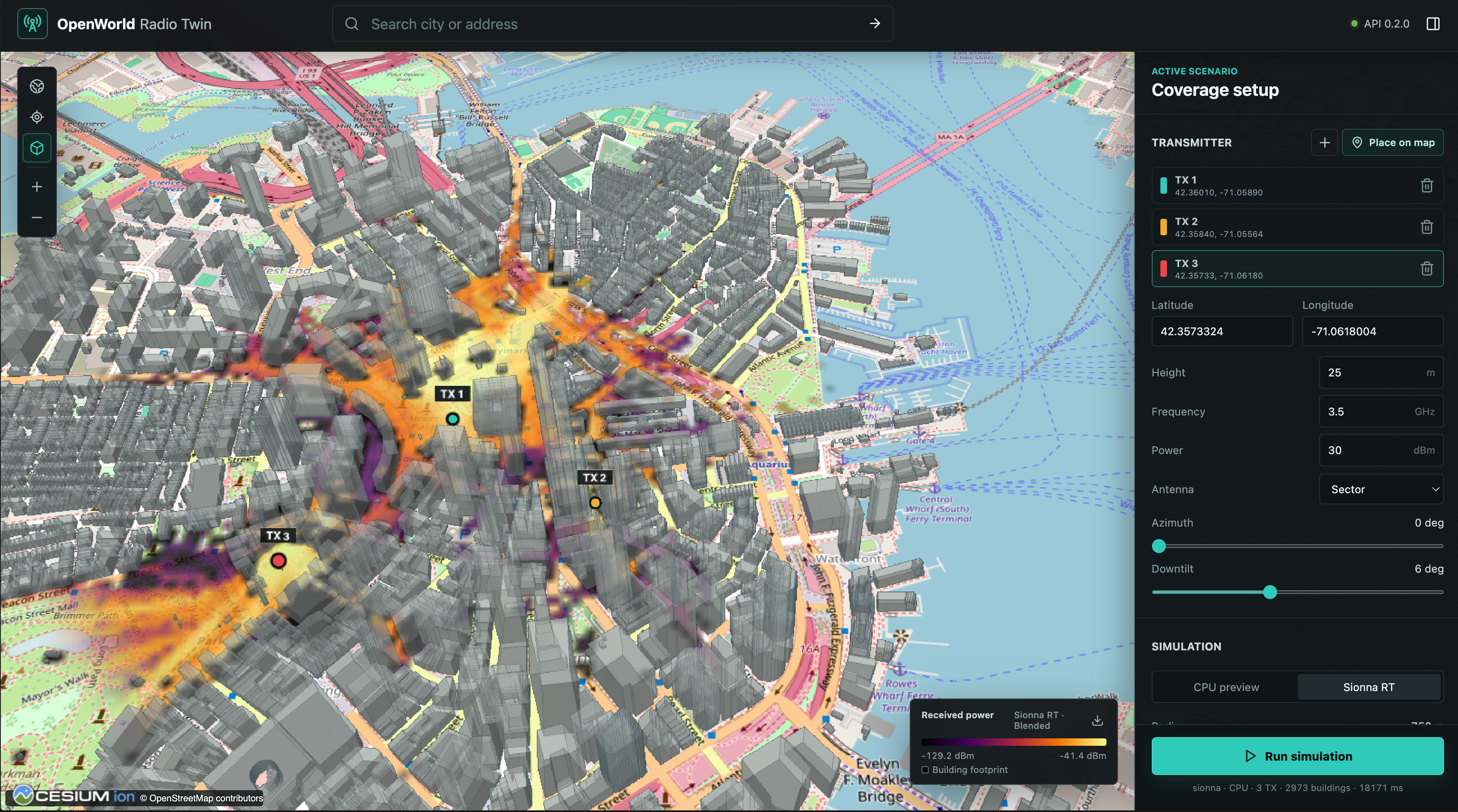
The explorer at / shows one continuous CesiumJS globe. Spatial tiles are an implementation detail of providers and caches; users never select a simulation tile. A simulation builds the region around the scene centre and returns the result in WGS84 coordinates on the same globe.

Navigation

• Search finds a city or an address through Nominatim.

• Orbit, pan, tilt and zoom freely; World view, Focus transmitter and Toggle 3D angle switch between overview, transmitter-centred, top-down and oblique views.

• The globe has relief everywhere. Its display terrain streams from Mapzen Terrain Tiles on AWS Open Data, the same Tilezen product family as the Skadi elevations the compiler samples outside the United States. Display heights never enter a scene or a dataset; they only position what the explorer draws.

• Buildings stream in around the camera from the selected source, up to the browsing limit (OWRT_MAX_VIEW_BUILDINGS), and the status line reports the provider, count and whether the limit was reached. These context buildings rest on the display terrain.

Compiled scenes

The explorer follows the Python workflow: define a scene, compile it, place transmitters inside it, solve. The page opens with no scene and no transmitter. A scene centre comes from one of three actions: drawing an area on the map, choosing a search result, or loading an example from the Scene section. Compile scene then calls POST /api/scenes with that centre and the geometry controls. The service runs the same compile_cached_scene call that owrt.load_scene uses, so the scene lands in the shared cache under the same directory name, and a scene compiled from Python appears in the explorer as a cache hit.

Inside the square the globe is clipped away and replaced by the compiled scene: the terrain grid with its levelled water, the surface classes as a tint over the base map, the building meshes at their solver positions, and a dashed boundary line. Outside the square the display globe continues. The inset is anchored to the display terrain at the scene origin, so the two meet along the boundary with only their resampling differences.

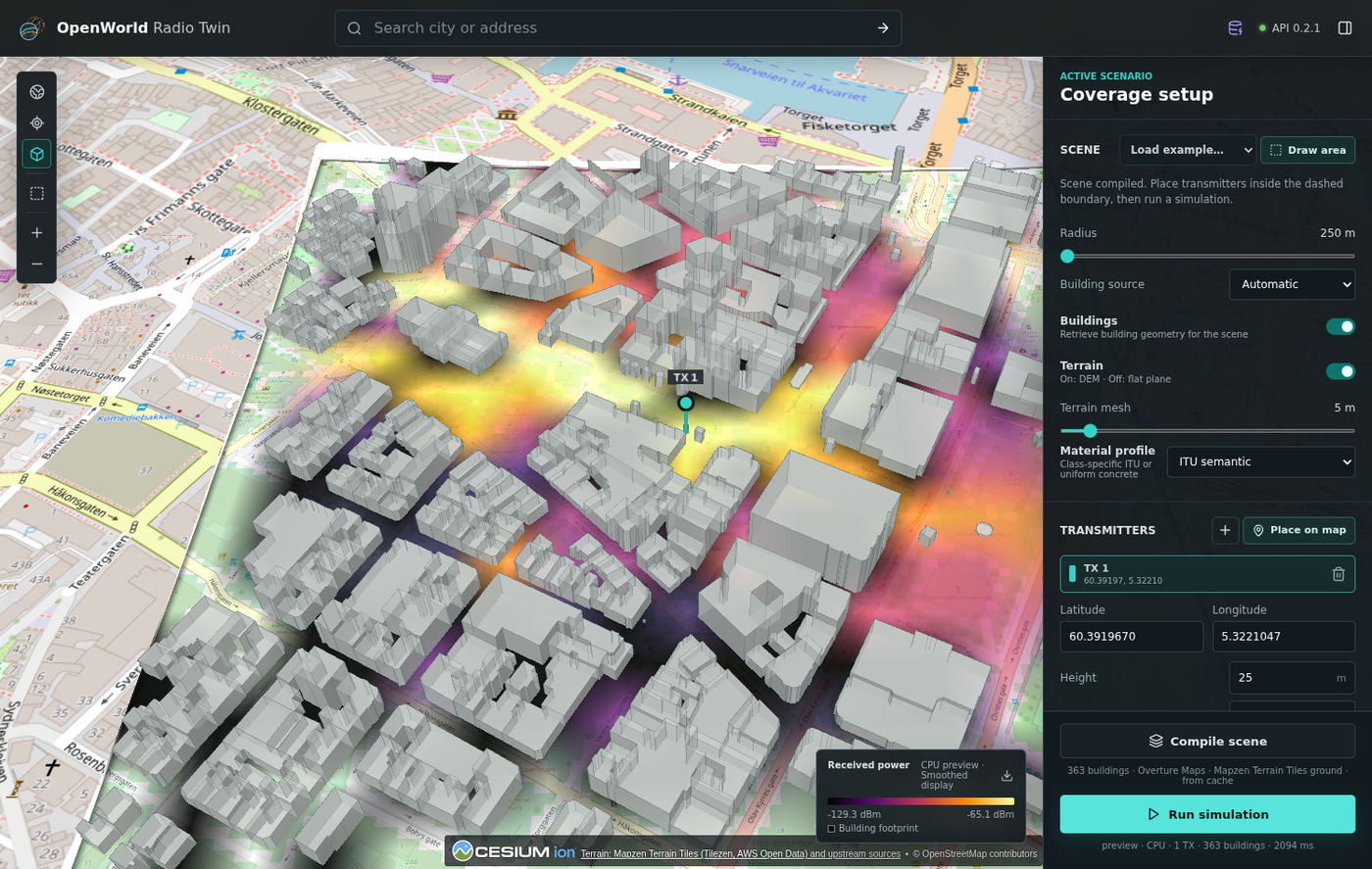
A compiled Bergen scene in the explorer: the scene terrain with its surface-class tint and buildings replaces the globe inside the dashed boundary, and the coverage layer follows it.

Draw area enters a drawing mode: drag a diagonal on the globe and the outline snaps to the square that will be compiled, with its side length shown. On release the centre and radius are taken from the square and the scene compiles at once. Esc or the banner’s close button cancels. Transmitters that fall outside a newly compiled square are removed.

The status line under the button names the building provider, the ground source and whether the scene came from the cache. Changing a scene input after compiling marks the status as stale; Run simulation compiles again on demand, so the extra step is never required.

Transmitters

Transmitters are added after a scene is compiled and must lie inside its square, as scene.add follows load_scene in Python. Place on map enters a placement mode in which a click inside the dashed boundary creates the first transmitter or moves the selected one; a click outside is refused. Add transmitter appends an entry at the scene centre, up to eight, each with its own latitude, longitude, height above ground, frequency, power, antenna pattern (Sector or Isotropic), azimuth and downtilt. The scene origin is the compiled centre, not a transmitter.

Simulation panel

Control	Effect
Engine	CPU preview or Sionna RT; Sionna RT shows its runtime message when the runtime is not installed
Solver parameters	Ray depth, samples per transmitter and propagation switches for Sionna RT
Radius	Scene half-width, 100 m to 5 km
Resolution	Receiver cell size in metres
Building source	Automatic, Global, or a specific source (Building sources)
Buildings	Include building geometry
Terrain mesh and spacing	DEM-following ground and its mesh spacing
Material profile	ITU semantic classes or Uniform material
Receiver plane height	Height above ground of the measurement surface

Run simulation is enabled once a compiled scene holds at least one transmitter. It posts the request with the scene centre to POST /api/simulations; the service compiles or reuses the scene, runs the solve on the persisted scene assets, and returns the coverage layer, the scene payload, warnings, solver details and provenance.

Coverage layers

Switch between Path gain, RSS, SINR and Association with the metric buttons. The layer is fetched from GET /api/simulations/{id}/raster.png and draped at the receiver height above the scene terrain. Smooth coverage applies display-only filtering with a boundary fade; the exact mode shows one pixel per solver cell. Mask buildings hides cells under building footprints. Surface classes toggles the class tint on the scene ground. Vertical exaggeration scales displayed relief on the globe and in the scene alike; at zero everything is flat, which shows what a scene compiled without terrain would look like. Both are display controls and change nothing in the exported arrays. The legend shows the display range and which solver produced the result.

Downloads

Download result bundle fetches GET /api/simulations/{id}/artifacts.zip, the bundle described in Exports. Results are kept in memory for the most recent simulations only; a download after the result has expired returns a 404.