Resolution and ray budget

The requested resolution maps directly to Sionna RT’s RadioMapSolver.cell_size in metres: it is the physical receiver-grid spacing. samples_per_tx is a per-transmitter budget; the solver launches samples_per_tx × transmitter_count initial samples. Increasing the budget does not subdivide a coarse cell, and refining the cell does not add samples.

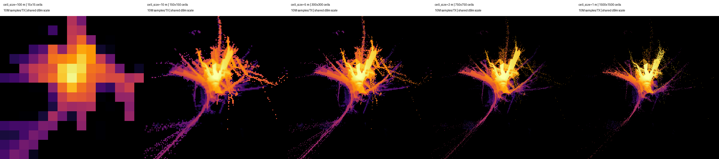
The same Boston scene and transmitter with only cell_size changed. Pixels are copied from native cells for display; no numerical interpolation is written.

Cell size	Native grid for a 750 m radius	Receiver cells
100 m	15 × 15	225
10 m	150 × 150	22,500
5 m	300 × 300	90,000
2 m	750 × 750	562,500
1 m	1,500 × 1,500	2,250,000

The last row is the Sionna grid limit of 2,250,000 receiver cells. The comparison shows spatial discretisation, not convergence; finer grids need an appropriate budget and a convergence check. At a fixed cell size, doubling the radius creates about four times as many cells, so the diagnostic ratio samples_per_tx / receiver_cells recorded with each result falls by about four. The ratio is not a measured hit count, because path intersections are not uniformly distributed. Adding transmitters does not divide the per-TX budget but increases total work and can introduce real association and SINR boundaries.

Display versus data

The browser receives one pixel per cell. Smooth coverage applies linear screen filtering and a boundary fade for display only; turning it off shows exact cells. Neither mode recomputes or exports interpolated values. Raw linear arrays remain the source of truth; PNGs are georeferenced renderings whose metadata records the source grid, units, display range and integer display scale.