Geographic scenes for Sionna RT

This tutorial turns a WGS84 location into a native sionna.rt.Scene with buildings, terrain, and semantic ground surfaces (water, vegetation, pavement, bare ground), then runs a standard Sionna RT radio-map workflow on it. Compared with a regular Sionna notebook, only the scene-loading line changes. Antenna arrays, radio devices, RadioMapSolver, scene.preview(), and scene.render() are the unmodified upstream API.

Outline

1. Setup

2. Load a geographic scene

3. Inspect the compiled geometry, materials, and provenance

4. Preview the scene in interactive 3D

5. Place a transmitter with geographic coordinates

6. Compute a terrain-following radio map

7. Preview the radio map in interactive 3D

8. Analyse the radio map quantitatively

9. Compare environments: materials, terrain, buildings

10. Georeference the results

Requirements. Sionna RT 2.0.x with a working Mitsuba backend (CUDA or LLVM CPU) and the notebook extras:

pip install -e ".[rt,tutorial]"

The first run for a location downloads public building, terrain, and land-cover data and compiles a scene into a local cache; later runs reuse it. Every parameter below is set to its highest-fidelity value: 1 m terrain mesh, 1 m receiver cells, 100 million rays per transmitter, depth 8, and a 1920 x 1200 viewer. The whole notebook, including the four-environment comparison, takes about ten minutes on a multi-core CPU, most of it geometry compilation, and a minute or two on a GPU. All 3D views are Sionna’s live interactive viewer, so their output exists only while a kernel is running.

1. Setup

Mitsuba’s execution variant is fixed per thread the first time it is selected. OWRT selects it from the device argument of load_scene, which is why sionna.rt is imported after the first load_scene call below. Everything else in this cell is an ordinary experiment definition.

import os
from pathlib import Path

import matplotlib.pyplot as plt
import numpy as np

from openworld_radio_twin import rt as owrt

DEVICE = "auto"  # "auto" | "cuda" | "cpu"
CACHE_DIR = Path(".cache/owrt-scenes")  # compiled scenes are reused across runs

# Amsterdam along the river Amstel: dense housing blocks, canals, and open water.
LOCATION = dict(latitude=52.3636, longitude=4.9019, radius_m=250)
TX_SITE = dict(latitude=52.3642, longitude=4.9030, height_agl=25.0)  # AGL: above ground level

FREQUENCY_HZ = 3.5e9
TX_POWER_DBM = 30.0
RX_HEIGHT_M = 1.5  # receiver height above the terrain
TERRAIN_RESOLUTION_M = 1.0  # terrain-mesh spacing
CELL_SIZE_M = 1.0  # receiver cell edge length
SAMPLES_PER_TX = 100_000_000
MAX_DEPTH = 8
SEED = 42

SCENE_VIEW = (1920, 1200)  # viewer size for the environment-only preview
RADIO_MAP_VIEW = (1920, 1080)  # a different size gives radio-map previews their own viewer

PATH_GAIN_LIMITS_DB = (-130.0, -70.0)  # one colour range for every path-gain figure

2. Load a geographic scene

owrt.load_scene accepts everything sionna.rt.load_scene accepts. Passing latitude, longitude, and radius_m instead of a filename compiles the square region centred on that point:

Argument	Values	Effect
buildings	"auto", "none"	Overture Maps buildings with an OpenStreetMap fallback, or no buildings
terrain	"elevation", "flat", "none"	DEM-based terrain, a plane at z = 0, or no ground at all
material_profile	"itu", "uniform"	ITU-R P.2040 materials per surface class, or itu_concrete everywhere
terrain_resolution_m	metres	Terrain-mesh spacing and DEM sampling
device	"auto", "cuda", "cpu"	Mitsuba variant, selected before sionna.rt is imported

The compiled scene is a plain Sionna XML file plus PLY meshes in a deterministic cache directory. The returned object is a sionna.rt.Scene, not a wrapper.

scene = owrt.load_scene(
    **LOCATION,
    buildings="auto",
    terrain="elevation",
    material_profile="itu",
    terrain_resolution_m=TERRAIN_RESOLUTION_M,
    cache_dir=CACHE_DIR,
    device=DEVICE,
)

import sionna.rt as rt  # noqa: E402 - the Mitsuba variant is now fixed

print(type(scene))
print("Scene directory:", os.path.relpath(owrt.scene_path(scene)))

<class 'sionna.rt.scene.Scene'>
Scene directory: .cache/owrt-scenes/scene_p52.36360_p4.90190_69617629838eaf426567

3. What was compiled

With the itu profile, each surface class carries a documented ITU-R P.2040 surrogate: bare ground is itu_medium_dry_ground, vegetation itu_wood, pavement and building walls itu_concrete, open water itu_wet_ground, and roofs itu_metal. Sionna merges shapes that share a material when it loads a scene, so the table below groups the scene by radio material. The river and the canals form the terrain-water object; building parts are merged into anonymous objects.

Everything here is a regular sionna.rt.SceneObject or RadioMaterial. Assigning a different RadioMaterial to scene.objects["terrain-water"].radio_material is the native way to test another water model.

ROLE = {
    "itu_medium_dry_ground": "exposed ground",
    "itu_wood": "vegetation",
    "itu_concrete": "building walls, paved ground",
    "itu_wet_ground": "open water (river, canals)",
    "itu_metal": "building roofs",
}

triangles = {}
for obj in scene.objects.values():
    material = obj.radio_material.name
    triangles[material] = triangles.get(material, 0) + obj.mi_mesh.face_count()

print(f"{'Radio material':<24}{'Role':<32}{'Triangles':>10}")
for material, count in sorted(triangles.items(), key=lambda item: -item[1]):
    print(f"{material:<24}{ROLE.get(material, ''):<32}{count:>10,}")
terrain_objects = sorted(name for name in scene.objects if name.startswith("terrain-"))
print(f"\nNamed terrain objects: {terrain_objects}")

Radio material          Role                             Triangles
itu_medium_dry_ground   exposed ground                     293,660
itu_wet_ground          open water (river, canals)         142,976
itu_concrete            building walls, paved ground        80,976
itu_metal               building roofs                       5,054
itu_wood                vegetation                             566

Named terrain objects: ['terrain-ground', 'terrain-vegetation', 'terrain-water']

Every compiled scene carries its data provenance. The summary below is read from the scene directory; the complete record, including licences and the ENU coordinate contract, is in provenance.json.

import json

scene_dir = owrt.scene_path(scene)
compilation = json.loads((scene_dir / "scene_info.json").read_text())["provenance"]
terrain_info = json.loads((scene_dir / "terrain" / "scene_info.json").read_text())

print(
    f"Buildings : {compilation['exported_building_count']} from {compilation['building_provider']} "
    f"{compilation['building_release']} "
    f"({compilation['boundary_excluded_building_count']} crossing the scene boundary were excluded)"
)
print(
    f"Terrain   : {terrain_info['terrain_source']['provider']}, "
    f"{terrain_info['terrain_source']['source_resolution_m']:.0f} m source resolution"
)
surface_source = terrain_info["surface_source"]
print(f"Surfaces  : {surface_source['provider']} {surface_source['release']}")
print("Warnings  :")
for warning in compilation["warnings"]:
    print("  -", warning)

Buildings : 736 from Overture Maps 2026-08-19.0 (92 crossing the scene boundary were excluded)
Terrain   : Mapzen Terrain Tiles, 31 m source resolution
Surfaces  : Overture Maps 2026-08-19.0
Warnings  :
  - Excluded 92 building footprints crossing the square scene boundary.
  - Global terrain uses a multi-source Mapzen mosaic; regional source accuracy, datum consistency, and attribution must be reviewed in exported metadata.
  - 100 road sections lacked source width; deterministic class widths are recorded as assumptions.
  - 25 road sections lacked source surface; deterministic road-class surfaces are recorded as assumptions.

4. Preview the scene in interactive 3D

scene.preview() is Sionna’s interactive viewer, built on ipywidgets and pythreejs. It shows the complete compiled geometry at full resolution: drag to orbit, scroll to zoom, right-drag to pan, and Alt+click to read a point’s coordinates. Water is drawn in blue, vegetation in green, bare ground in brown, and buildings in grey. This first view contains no radio map; it is the place to check the river, the canals, the terrain, and the building footprints before any transmitter is added.

JupyterLab renders the widget out of the box. VS Code has to be allowed to fetch the widget’s JavaScript: add the following to your settings, reload the window, and restart the kernel.

"jupyter.widgetScriptSources": ["jsdelivr.com", "unpkg.com"]

The widget lives in the running kernel and is not stored in the committed notebook. For a paper figure, scene.render_to_file(camera="preview", filename=...) traces the current viewer pose with Mitsuba’s path tracer.

Sionna keeps one cached viewer per scene and redraws it in place on every preview() call, so a later call with a radio map would also change this output. Requesting a different resolution makes Sionna create an independent viewer; that is why the radio-map previews below use RADIO_MAP_VIEW while this one uses SCENE_VIEW.

scene.preview(resolution=SCENE_VIEW)

5. Place a transmitter with geographic coordinates

Sionna positions radio devices in metres in the scene frame. OWRT’s frame is topocentric east-north-up at the scene centre, with z = 0 at the modelled terrain elevation of that centre. owrt.position converts latitude, longitude, and a height above ground level into that frame, terrain included. The device itself is a standard sionna.rt.Transmitter; any Sionna antenna array works.

scene.frequency = FREQUENCY_HZ
scene.tx_array = rt.PlanarArray(num_rows=1, num_cols=1, pattern="iso", polarization="V")
scene.rx_array = rt.PlanarArray(num_rows=1, num_cols=1, pattern="iso", polarization="V")

tx_position = owrt.position(scene, **TX_SITE)
scene.add(rt.Transmitter(name="tx", position=tx_position, power_dbm=TX_POWER_DBM))

east, north, z = tx_position
print(f"Transmitter in scene coordinates: east {east:.1f} m, north {north:.1f} m, z {z:.2f} m")
print(
    f"Terrain under the transmitter: {owrt.terrain_elevation(scene, east, north):.2f} m, "
    f"antenna {TX_SITE['height_agl']:.1f} m above it"
)

Transmitter in scene coordinates: east 74.9 m, north 66.8 m, z 26.61 m
Terrain under the transmitter: 1.61 m, antenna 25.0 m above it

6. Compute a terrain-following radio map

Sionna’s default radio-map surface is a horizontal plane. Over real terrain the receivers should follow the ground, which Sionna supports through the measurement_surface argument of RadioMapSolver (see Radio Maps in the Sionna documentation). owrt.measurement_surface builds that mesh: a regular grid whose every vertex sits height metres above the local terrain, two triangles per cell. The solver call is unchanged Sionna.

measurement_surface = owrt.measurement_surface(scene, cell_size=CELL_SIZE_M, height=RX_HEIGHT_M)
print(
    f"Measurement surface: {measurement_surface.face_count():,} triangles, "
    f"two per {CELL_SIZE_M:g} m x {CELL_SIZE_M:g} m cell, {RX_HEIGHT_M} m above the terrain"
)

solver = rt.RadioMapSolver()
radio_map = solver(
    scene,
    measurement_surface=measurement_surface,
    samples_per_tx=SAMPLES_PER_TX,
    max_depth=MAX_DEPTH,
    seed=SEED,
)
print(f"{type(radio_map).__name__} with {radio_map.cells_count:,} cells")

Measurement surface: 500,000 triangles, two per 1 m x 1 m cell, 1.5 m above the terrain
MeshRadioMap with 500,000 cells

7. Preview the radio map in interactive 3D

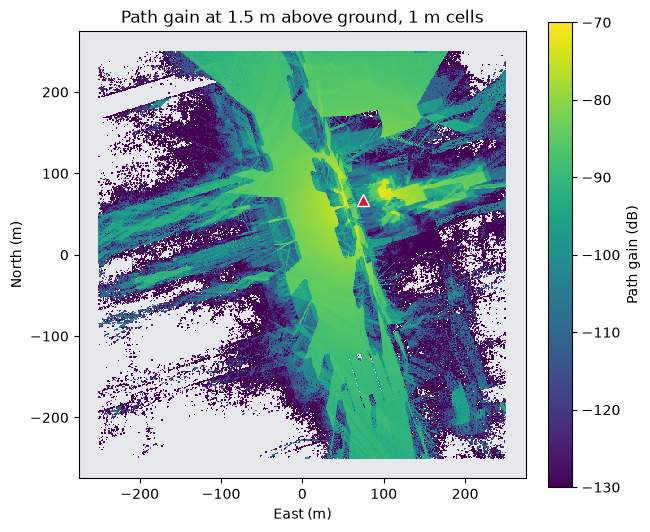
The same viewer accepts the radio map and drapes it over the terrain-following measurement surface, one colour per 1 m cell. rm_metric selects "path_gain", "rss", or "sinr", and fixed rm_vmin/rm_vmax keep the colour scale identical across figures. This notebook displays path gain, the quantity that depends only on the environment; with a single transmitter, RSS in dBm is path gain plus the transmit power.

If you also call scene.render(radio_map=..., rm_metric="rss"): in Sionna RT 2.0.1 it can scale the radio map in place by a factor of 1000 when a transmitter radiates exactly 1 W (30 dBm), because the dBm conversion is applied to a zero-copy view of the path-gain tensor. Rendering "path_gain" avoids this.

scene.preview(
    radio_map=radio_map,
    rm_metric="path_gain",
    rm_vmin=PATH_GAIN_LIMITS_DB[0],
    rm_vmax=PATH_GAIN_LIMITS_DB[1],
    resolution=RADIO_MAP_VIEW,
)

8. Analyse the radio map quantitatively

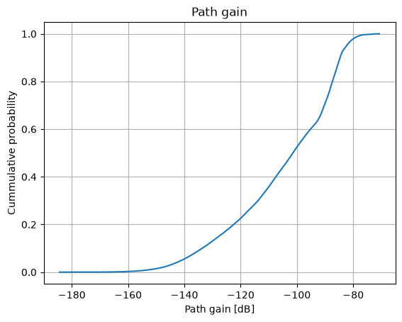
radio_map.cdf() is native. For a top-down map, Sionna provides show() only for planar radio maps; a mesh radio map holds one value per triangle, so it is plotted with Matplotlib’s tripcolor straight from radio_map.measurement_surface. The two helpers below work for any MeshRadioMap, not only for OWRT scenes.

radio_map.cdf(metric="path_gain");

def metric_db(radio_map, metric="path_gain"):
    """Strongest-transmitter value per triangle in dB (dBm for RSS); NaN where no path arrived."""
    linear = radio_map.transmitter_radio_map(metric).numpy()
    offset = 30.0 if metric == "rss" else 0.0
    with np.errstate(divide="ignore"):
        return np.where(linear > 0, 10.0 * np.log10(linear) + offset, np.nan)


def show_mesh_radio_map(
    scene,
    radio_map,
    values_db,
    *,
    ax=None,
    label="Path gain (dB)",
    cmap="viridis",
    vmin=None,
    vmax=None,
):
    """Plot one value per measurement-surface triangle; grey marks missing coverage."""
    mesh = radio_map.measurement_surface
    vertices = np.asarray(mesh.vertex_positions_buffer()).reshape(-1, 3)
    faces = np.asarray(mesh.faces_buffer()).reshape(-1, 3)
    if ax is None:
        _, ax = plt.subplots(figsize=(6.4, 5.6), constrained_layout=True)
    ax.set_facecolor("#e6e8eb")
    image = ax.tripcolor(
        vertices[:, 0], vertices[:, 1], faces, facecolors=values_db, cmap=cmap, vmin=vmin, vmax=vmax
    )
    for tx in scene.transmitters.values():
        x, y, _ = tx.position.numpy().ravel()
        ax.plot(x, y, "^", color="crimson", markersize=9, markeredgecolor="white")
    ax.set_aspect("equal")
    ax.set_xlabel("East (m)")
    ax.set_ylabel("North (m)")
    ax.figure.colorbar(image, ax=ax, label=label, shrink=0.85)
    return ax

path_gain_db = metric_db(radio_map)

ax = show_mesh_radio_map(
    scene, radio_map, path_gain_db, vmin=PATH_GAIN_LIMITS_DB[0], vmax=PATH_GAIN_LIMITS_DB[1]
)
ax.set_title(f"Path gain at {RX_HEIGHT_M} m above ground, {CELL_SIZE_M:g} m cells")

covered = np.isfinite(path_gain_db)
print(f"Covered cells: {covered.mean():.1%}")
print(f"Median path gain over covered cells: {np.nanmedian(path_gain_db):.1f} dB")

Covered cells: 65.2%
Median path gain over covered cells: -101.5 dB

9. Compare environments: materials, terrain, buildings

Because the environment is described by keyword arguments, an ablation is a second load_scene call with one argument changed. The transmitter, arrays, solver settings, and receiver grid stay identical, and every variant’s measurement grid has the same triangle order, so per-cell differences are well defined. Each variant is its own Scene, so each one also gets its own interactive viewer.

Scenario	Change	Isolates
ITU materials	none (the scene above)	reference
Uniform concrete	material_profile="uniform"	semantic materials: water, vegetation, ground
Flat terrain	terrain="flat"	terrain relief and the semantic surfaces that come with it
No buildings	buildings="none"	building geometry

def solve_variant(**scene_options):
    """Load a variant of LOCATION and solve it with the radio configuration used above."""
    variant = owrt.load_scene(
        **LOCATION,
        terrain_resolution_m=TERRAIN_RESOLUTION_M,
        cache_dir=CACHE_DIR,
        device=DEVICE,
        **scene_options,
    )
    variant.frequency = FREQUENCY_HZ
    variant.tx_array = rt.PlanarArray(num_rows=1, num_cols=1, pattern="iso", polarization="V")
    variant.rx_array = rt.PlanarArray(num_rows=1, num_cols=1, pattern="iso", polarization="V")
    variant.add(
        rt.Transmitter(
            name="tx", position=owrt.position(variant, **TX_SITE), power_dbm=TX_POWER_DBM
        )
    )
    surface = owrt.measurement_surface(variant, cell_size=CELL_SIZE_M, height=RX_HEIGHT_M)
    variant_map = solver(
        variant,
        measurement_surface=surface,
        samples_per_tx=SAMPLES_PER_TX,
        max_depth=MAX_DEPTH,
        seed=SEED,
    )
    return variant, variant_map


SCENARIOS = {
    "ITU materials": {},
    "Uniform concrete": dict(material_profile="uniform"),
    "Flat terrain": dict(terrain="flat"),
    "No buildings": dict(buildings="none"),
}

results = {"ITU materials": (scene, radio_map)}
for name, options in SCENARIOS.items():
    if name not in results:
        results[name] = solve_variant(**options)
maps_db = {name: metric_db(variant_map) for name, (_, variant_map) in results.items()}

One interactive viewer per scenario, all on the same colour scale. Orbit each one to compare how the river, the terrain, and the buildings shape the coverage.

for name, (variant, variant_map) in results.items():
    print(name)
    variant.preview(
        radio_map=variant_map,
        rm_metric="path_gain",
        rm_vmin=PATH_GAIN_LIMITS_DB[0],
        rm_vmax=PATH_GAIN_LIMITS_DB[1],
        resolution=RADIO_MAP_VIEW,
    )

ITU materials
Uniform concrete
Flat terrain
No buildings

The quantitative view: top row, path gain per scenario on a shared scale; bottom row, the distribution over covered cells and each variant’s per-cell difference to the reference.

reference_db = maps_db["ITU materials"]
fig, axes = plt.subplots(2, len(maps_db), figsize=(5.4 * len(maps_db), 10), constrained_layout=True)

for column, (name, values_db) in enumerate(maps_db.items()):
    variant, variant_map = results[name]
    show_mesh_radio_map(
        variant,
        variant_map,
        values_db,
        ax=axes[0, column],
        vmin=PATH_GAIN_LIMITS_DB[0],
        vmax=PATH_GAIN_LIMITS_DB[1],
    )
    axes[0, column].set_title(name)
    if column == 0:
        continue
    delta_db = values_db - reference_db
    limit = float(np.nanpercentile(np.abs(delta_db), 98))
    show_mesh_radio_map(
        variant,
        variant_map,
        delta_db,
        ax=axes[1, column],
        cmap="RdBu_r",
        vmin=-limit,
        vmax=limit,
        label="Difference to reference (dB)",
    )
    axes[1, column].set_title(f"{name} minus ITU materials")

for name, values_db in maps_db.items():
    covered_db = np.sort(values_db[np.isfinite(values_db)])
    axes[1, 0].plot(covered_db, np.linspace(0, 1, covered_db.size), label=name)
axes[1, 0].set(xlabel="Path gain (dB)", ylabel="CDF over covered cells", title="Distribution")
axes[1, 0].grid(alpha=0.3)
axes[1, 0].legend()

print(f"{'Scenario':<18}{'Covered':>9}{'Median (dB)':>13}{'Median |diff|':>15}{'95% |diff|':>12}")
for name, values_db in maps_db.items():
    delta_db = np.abs(values_db - reference_db)
    diff = (
        "reference".rjust(27)
        if name == "ITU materials"
        else (f"{np.nanmedian(delta_db):>15.2f}{np.nanpercentile(delta_db, 95):>12.2f}")
    )
    print(f"{name:<18}{np.isfinite(values_db).mean():>8.1%}{np.nanmedian(values_db):>13.1f}{diff}")

Scenario            Covered  Median (dB)  Median |diff|  95% |diff|
ITU materials        65.2%       -101.5                  reference
Uniform concrete     65.6%       -100.8           0.54       16.94
Flat terrain         63.3%       -101.8           1.58       23.11
No buildings         96.9%        -88.9          15.12       52.90

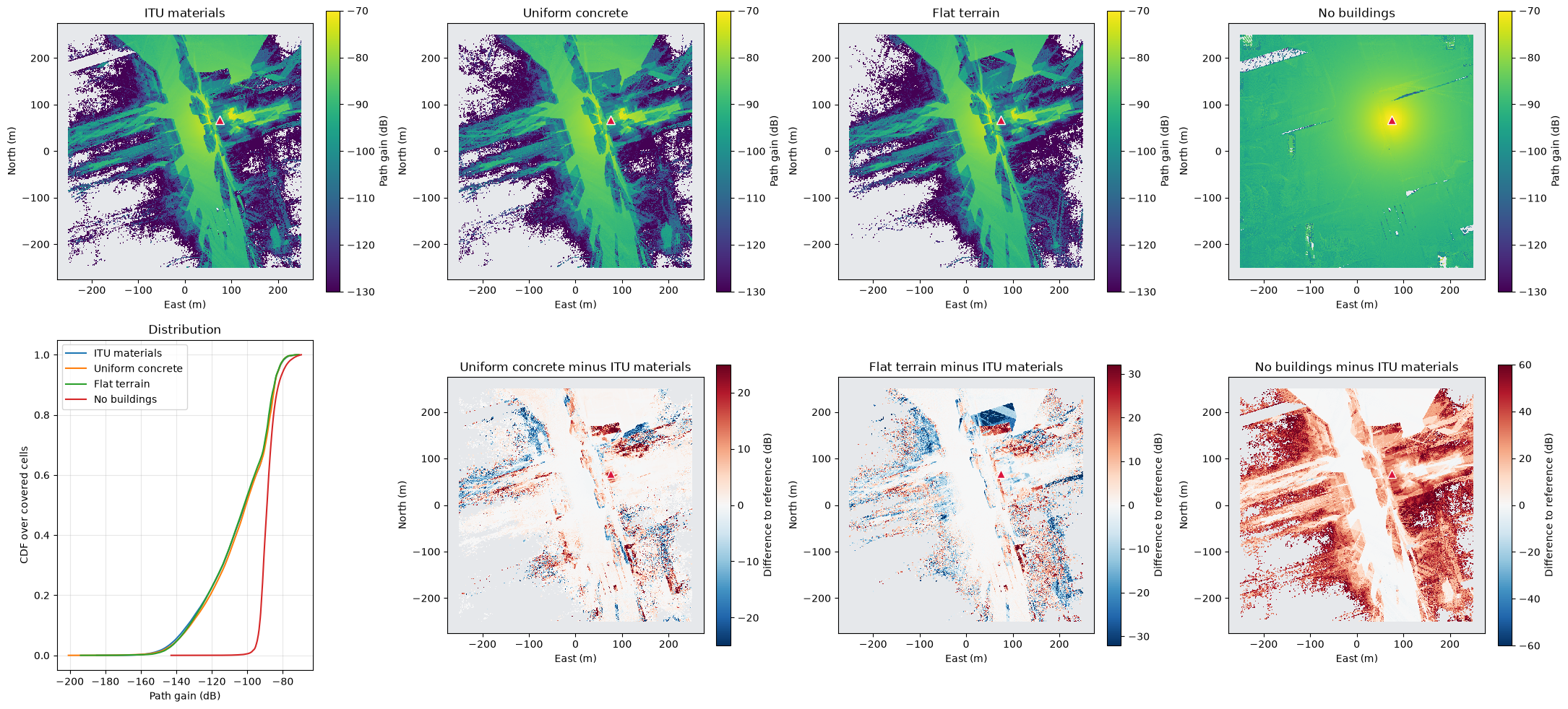
These statistics describe one ray-tracing run per scenario. Before reporting a difference as a result, repeat with several seeds and quantify the spread; the sample budget is already at 100 million rays per transmitter.

10. Georeference the results

Everything so far is in scene metres. owrt.scene_frame returns the WGS84-to-ENU transform of the scene, so any cell centre or device position converts back to latitude and longitude. The measurement grid also has a fixed layout, documented in the sidecar next to the mesh: triangles 2k and 2k+1 belong to cell k = row * columns + column, with rows running south to north and columns west to east. A mesh radio map therefore reshapes into a raster without a lookup table.

import math

frame = owrt.scene_frame(scene)
centers = radio_map.cell_centers
strongest = int(np.nanargmax(path_gain_db))
longitude, latitude, _ = frame.to_geographic(
    float(centers.x.numpy()[strongest]), float(centers.y.numpy()[strongest])
)
print(f"Strongest cell: {latitude:.6f} N, {longitude:.6f} E, {path_gain_db[strongest]:.1f} dB")

columns = rows = math.ceil(2 * LOCATION["radius_m"] / CELL_SIZE_M)
cell_linear = (
    radio_map.transmitter_radio_map("path_gain").numpy().reshape(rows, columns, 2).mean(axis=-1)
)
with np.errstate(divide="ignore"):
    raster_db = np.where(cell_linear > 0, 10.0 * np.log10(cell_linear), np.nan)
print(f"Raster: {raster_db.shape} cells; row 0 is the south edge, column 0 the west edge")

west, south = frame.to_geographic(-LOCATION["radius_m"], -LOCATION["radius_m"])[:2]
east_, north_ = frame.to_geographic(LOCATION["radius_m"], LOCATION["radius_m"])[:2]
print(f"Raster bounds: {south:.6f} N to {north_:.6f} N, {west:.6f} E to {east_:.6f} E")

Strongest cell: 52.364244 N, 4.903329 E, -70.7 dB
Raster: (500, 500) cells; row 0 is the south edge, column 0 the west edge
Raster bounds: 52.361353 N to 52.365847 N, 4.898230 E to 4.905570 E

Reproducibility notes

• Cache. Scenes are keyed by the compiler version and the geometry arguments (latitude, longitude, radius_m, buildings, terrain, material_profile, terrain_resolution_m). Frequency, arrays, transmitters, receiver grids, and solver settings never trigger a recompile. The cache root is cache_dir, else OWRT_SCENE_CACHE_ROOT, else .cache/scenes under the checkout.

• Offline use. owrt scene compile --lat 52.3636 --lon 4.9019 --radius 250 --output scenes/amstel writes the same directory layout. Its scene.xml loads with plain sionna.rt.load_scene; passing the directory to owrt.load_scene keeps the geographic helpers available.

• Provenance. provenance.json records the data sources, their releases and licences, the coordinate contract, and the material profile. Cite the sources listed there together with Sionna RT.

• Fidelity. The notebook already runs at 1 m terrain and receiver resolution with 100 million rays per transmitter. The terrain source itself is coarser (about 31 m for this location), so the 1 m mesh oversamples it; building footprints and the semantic surfaces are the parts that benefit. Raise LOCATION["radius_m"] for a larger district and use a GPU (device="cuda") to keep the turnaround short. Sionna’s own tutorials on paths, multi-transmitter coverage, and differentiable ray tracing apply to these scenes without modification.