
Radio maps as a PyTorch dataset#
RadioMapDataset reads the radio maps of an OWRT-RF package as PyTorch samples: the scene geometry on the radio grid, the transmitters, and the per-transmitter path gain that Sionna computed, with the received power (RSS) and the signal-to-interference-plus-noise ratio (SINR) derived from it. This tutorial reads the sample package in both of the dataset’s modes, selects radio maps by split and by index query, batches random crops, and trains a small convolutional network for a few steps. It then evaluates the network on the validation split and derives SINR and the serving transmitter from its predictions. Everything runs on a CPU.
Outline
Setup
The index of a package
Whole radio maps
One transmitter per sample
Selecting radio maps
DataLoader settings
Random crops for batching
Inputs and normalisation
Train a small model
Evaluate on the validation split
SINR and the serving transmitter from predictions
1. Setup#
The dataset needs the torch extra. The notebook also uses Jupyter, and pandas to show the index as a table, from the tutorial extra:
python -m pip install -e ".[torch,tutorial]"
ROOT is a package directory with its scene archives extracted into it. A package is a release of radio maps, or the output of owrt dataset package on a dataset you generated (see Packaging for release in the dataset guide). [Download location of the OWRT-RF sample package: to be added when it is published.] Check and extract a package once, inside the package directory:
sha256sum -c SHA256SUMS
for archive in scenes/*.tar.zst; do tar --zstd -xf "$archive"; done
GNU tar before 1.31 takes -I zstd instead of --zstd. The sample package takes about 0.54 GB as archives and about 1.1 GB more once extracted. The environment variable OWRT_RF_ROOT overrides the default location below. A relative location is relative to the kernel’s working directory, which Jupyter sets to the notebook’s folder. The default is therefore data/owrt-rf-sample next to the notebook, examples/data/owrt-rf-sample in the repository.
The stored outputs come from the OWRT-RF sample package. On the machine that produced them, two 16-core CPUs with 64 hardware threads, the notebook took about seven minutes, half of it the training in section 9. The figures are stored as SVG, with vector lines, markers and text. To keep the notebook small, the maps show every third cell in each direction, each pixel centred on the cell it shows. The setup cell prints the PyTorch and OpenWorld Radio Twin versions that ran the notebook and the number of PyTorch threads, and section 2 the version that wrote the package.
# SVG figures: lines, markers and text stay vectors; imshow(interpolation="none") embeds one pixel per cell.
%config InlineBackend.figure_formats = ["svg"]

import os
import time
from pathlib import Path

import matplotlib.patheffects as patheffects
import matplotlib.pyplot as plt
import numpy as np
import pandas as pd
import pyarrow.compute as pc
import torch
from matplotlib.colors import ListedColormap
from torch.utils.data import DataLoader

import openworld_radio_twin
from openworld_radio_twin.torch_dataset import RadioMapDataset, RandomCrop

# An OWRT-RF package with its scene archives extracted into it.
ROOT = Path(os.environ.get("OWRT_RF_ROOT", "data/owrt-rf-sample"))
if not (ROOT / "index.parquet").is_file():
    raise FileNotFoundError(f"No OWRT-RF package in {ROOT}; set OWRT_RF_ROOT to an extracted package directory")

SEED = 0
CROP = 256  # cells per side of a training crop
BATCH_SIZE = 8
WORKERS = 4  # DataLoader workers; 0 reads in the main process
STEPS = 150  # training steps
MAP_STEP = 3  # figures show every third cell in each direction, to keep the notebook small

torch.manual_seed(SEED)
pd.set_option("display.width", 120)
print(f"torch {torch.__version__} with {torch.get_num_threads()} threads, openworld_radio_twin {openworld_radio_twin.__version__}")
torch 2.14.0+cpu with 32 threads, openworld_radio_twin 0.3.0
2. The index of a package#
Every RadioMapDataset reads the package’s index.parquet, one row per radio map, and refuses an index that is out of date with the package manifest. index holds the rows of the selected radio maps as a pyarrow.Table; pandas shows it as a table. The package splits by scene, never by radio map, and overlapping scenes, and scenes of one site, share a split. The validation and test scenes therefore share no geometry with the training scenes. The Parquet footer of the index records the dataset format and the version that wrote the package.
radio_maps = RadioMapDataset(ROOT)
index = radio_maps.index.to_pandas()
print(f"{len(radio_maps)} radio maps with {index['n_tx'].sum()} transmitters in {index['scene'].nunique()} scenes")
footer = {key.decode(): value.decode() for key, value in radio_maps.index.schema.metadata.items()}
print(f"Dataset format {footer['owrt.schema_version']}, written by openworld_radio_twin {footer['owrt.openworld_radio_twin_version']}")

index.groupby(["split", "label"], sort=False).agg(
    radio_maps=("name", "size"),
    tx_per_map=("n_tx", list),
    buildings=("building_source", "first"),
    terrain=("terrain_provider", "first"),
)
24 radio maps with 155 transmitters in 6 scenes
Dataset format 2, written by openworld_radio_twin 0.3.0
| radio_maps | tx_per_map | buildings | terrain | ||
|---|---|---|---|---|---|
| split | label | ||||
| validation | Amsterdam centre | 4 | [5, 6, 8, 5] | 3dbag | Mapzen Terrain Tiles |
| test | Berlin Potsdamer Platz | 4 | [8, 7, 5, 8] | berlin | Mapzen Terrain Tiles |
| train | Paris Champ de Mars | 4 | [7, 5, 6, 8] | global | Mapzen Terrain Tiles |
| San Francisco Embarcadero | 4 | [5, 7, 4, 8] | global | USGS 3DEP | |
| Hong Kong Mid-Levels | 4 | [4, 7, 8, 8] | global | Mapzen Terrain Tiles | |
| Bergen Bryggen | 4 | [7, 6, 5, 8] | global | Mapzen Terrain Tiles |
The radio settings are the same in every radio map of the sample. The per-transmitter columns of the index are lists in transmitter order, shown here for the first radio map.
shared = ["engine", "frequency_hz", "bandwidth_hz", "resolution_m", "rows", "columns", "receiver_height_m", "samples_per_tx", "max_depth", "association_metric"]
print(index[shared].drop_duplicates().T.to_string(header=False))

first = index.iloc[0]
print(f"\n{first['radio_map_id']}")
print(pd.DataFrame({name: first[name] for name in ["tx_east_m", "tx_north_m", "tx_height_agl_m", "tx_power_dbm", "tx_azimuth_deg", "tx_downtilt_deg"]}).round(1).to_string())
engine                    sionna
frequency_hz        3500000000.0
bandwidth_hz           1000000.0
resolution_m                 1.0
rows                        1500
columns                     1500
receiver_height_m            1.5
samples_per_tx         100000000
max_depth                      8
association_metric          sinr

scene_001_amsterdam-centre/radio_map_0001_sector_5tx_3p5ghz
   tx_east_m  tx_north_m  tx_height_agl_m  tx_power_dbm  tx_azimuth_deg  tx_downtilt_deg
0      300.1      -172.6             21.4          34.6            81.4              1.5
1      661.4        16.1             25.1          24.2           152.2              8.6
2      556.0       325.5             20.1          34.1           123.9              9.9
3     -393.0      -493.1             27.3          34.5            10.8              2.4
4      114.8      -433.7             18.9          27.7            77.4              0.6
3. Whole radio maps#
By default one sample is one whole radio map with all its transmitters: a dictionary of tensors on the grid of the radio arrays. With T transmitters and H by W cells, rows run south to north and columns west to east.
sample = radio_maps[0]
for name, value in sample.items():
    kind = f"{str(value.dtype).removeprefix('torch.')} {tuple(value.shape)}" if torch.is_tensor(value) else type(value).__name__
    print(f"{name:<18}{kind}")
geometry          float32 (3, 1500, 1500)
surface_classes   int64 (1500, 1500)
indoor            bool (1500, 1500)
tx_map            float32 (5, 1500, 1500)
tx_cell           int64 (5, 2)
tx_position_m     float32 (5, 3)
tx_height_agl_m   float32 (5,)
tx_power_dbm      float32 (5,)
tx_azimuth_deg    float32 (5,)
tx_downtilt_deg   float32 (5,)
frequency_hz      float64 ()
coverage          bool (5, 1500, 1500)
path_gain_db      float32 (5, 1500, 1500)
rss_dbm           float32 (5, 1500, 1500)
sinr_db           float32 (5, 1500, 1500)
serving_tx        int64 (1500, 1500)
radio_map_id      str
The values keep their physical units; the dataset normalises nothing.
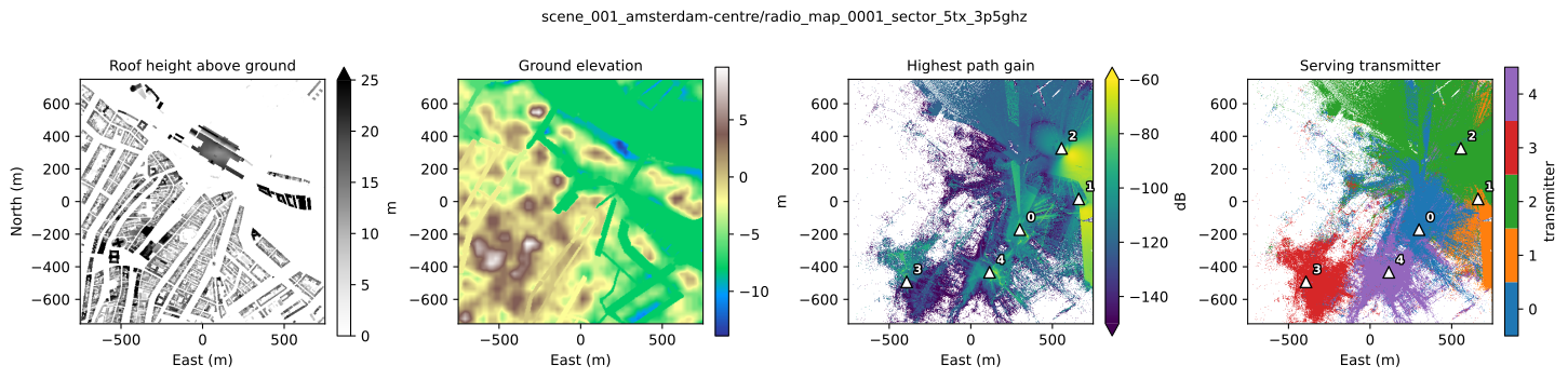
geometrystacks three channels: roof height above ground in metres (0 where there is no building), the building footprint mask, and the ground elevation in the scene frame in metres: the height of the measurement cell centre minus the receiver height.surface_classesholds the terrain class of each cell (here 0 ground, 1 vegetation, 2 paved, 3 water), andindoormarks receivers inside a building. A package of buildings on flat ground, such as the flat sampleowrt-rf-sample-flat, reads the same way, withsurface_classes-1 and the ground elevation 0 in every cell.tx_maphas a 1 in the cell of each transmitter.tx_cellgives that cell’s row and column, andtx_position_mthe east, north and up position in metres.path_gain_db,rss_dbmandsinr_dbare per transmitter, in dB and dBm.coverageis where the path gain, RSS and SINR are all positive. Outside it these arrays are 0, so a loss must usecoverageas its mask.serving_txis the index of the transmitter with the highest SINR, the recordedassociation_metric, and -1 where no transmitter reaches the cell.
coverage = sample["coverage"]
print("Covered cells per transmitter:", ", ".join(f"{value:.0%}" for value in coverage.float().mean((1, 2)).tolist()))
print(f"Indoor receivers: {sample['indoor'].float().mean():.0%}; cells with no serving transmitter: {(sample['serving_tx'] < 0).float().mean():.1%}")
print(f"Path gain outside coverage: {sample['path_gain_db'][~coverage].unique().tolist()} dB")
print(f"Path gain on covered cells: {sample['path_gain_db'][coverage].min():.1f} to {sample['path_gain_db'][coverage].max():.1f} dB")
Covered cells per transmitter: 22%, 14%, 29%, 9%, 14%
Indoor receivers: 29%; cells with no serving transmitter: 43.3%
Path gain outside coverage: [0.0] dB
Path gain on covered cells: -265.4 to -60.4 dB
The sample on a map in scene metres. Row 0 is the southern row, so the arrays are drawn with origin="lower"; triangles mark the transmitters at their recorded positions. Values beyond the ends of a colour bar take its end colours; the arrows mark this.
# The figures and the inputs of section 8 take these values from the first radio map.
GRID = ["radius_m", "row_step_m", "column_step_m", "receiver_height_m"]
assert index[GRID].nunique().eq(1).all() and (index["row_step_m"] == index["column_step_m"]).all()
assert (index["rows"] * index["row_step_m"] == 2 * index["radius_m"]).all() and (index["rows"] == index["columns"]).all()
RADIUS_M = float(index["radius_m"].iloc[0])
EXTENT = (-RADIUS_M, RADIUS_M, -RADIUS_M, RADIUS_M)  # the grid spans the scene square


def categories(count):
    # One colour per transmitter number, for maps of the serving transmitter.
    # tab10 without its grey, which would look like a missing value; turbo for more than nine.
    colours = [colour for i, colour in enumerate(plt.get_cmap("tab10").colors) if i != 7]
    colours = colours[:count] if count <= len(colours) else plt.get_cmap("turbo")(np.linspace(0, 1, count))
    return dict(cmap=ListedColormap(colours), vmin=-0.5, vmax=count - 0.5, ticks=range(count))


def show(ax, values, title, label, ticks=None, extend="neither", **style):
    # Every MAP_STEP-th cell in each direction, each pixel centred on the cell it shows; values beyond vmin or vmax take the end colours.
    first = MAP_STEP // 2
    cells = values[first::MAP_STEP, first::MAP_STEP]
    cell_m = 2 * RADIUS_M / values.shape[-1]
    west = -RADIUS_M + (first - (MAP_STEP - 1) / 2) * cell_m
    extent = (west, west + cells.shape[-1] * MAP_STEP * cell_m, west, west + cells.shape[-2] * MAP_STEP * cell_m)
    image = ax.imshow(cells, origin="lower", extent=extent, interpolation="none", **style)
    ax.set_title(title, fontsize=10)
    ax.set_xlabel("East (m)")
    ax.figure.colorbar(image, ax=ax, label=label, shrink=0.8, ticks=ticks, extend=extend)


OUTLINE = [patheffects.withStroke(linewidth=2, foreground="black")]


def mark_transmitters(ax, positions, numbers=None):
    numbers = range(len(positions)) if numbers is None else numbers
    for number, (east, north) in zip(numbers, positions[:, :2].tolist()):
        ax.plot(east, north, "^", color="white", markeredgecolor="black", markersize=8)
        # Near the east or north edge the label goes to the other side, inside the axes.
        right, up = east < RADIUS_M - 60, north < RADIUS_M - 40
        ax.annotate(str(number), (east, north), xytext=(5 if right else -5, 4 if up else -4), textcoords="offset points",
                    ha="left" if right else "right", va="bottom" if up else "top",
                    color="white", fontsize=8, fontweight="bold", path_effects=OUTLINE)


def missing(values, keep):
    return values.float().masked_fill(~keep, torch.nan)


best_gain = torch.where(coverage, sample["path_gain_db"], -torch.inf).amax(0)

fig, axes = plt.subplots(1, 4, figsize=(15, 3.6), constrained_layout=True)
show(axes[0], sample["geometry"][0], "Roof height above ground", "m", extend="max", cmap="Greys", vmin=0, vmax=25)
show(axes[1], sample["geometry"][2], "Ground elevation", "m", cmap="terrain")
show(axes[2], missing(best_gain, coverage.any(0)), "Highest path gain", "dB", extend="both", cmap="viridis", vmin=-150, vmax=-60)
show(axes[3], missing(sample["serving_tx"], sample["serving_tx"] >= 0), "Serving transmitter", "transmitter", **categories(len(sample["tx_position_m"])))
for ax in axes[2:]:
    mark_transmitters(ax, sample["tx_position_m"])
axes[0].set_ylabel("North (m)")
fig.suptitle(sample["radio_map_id"], fontsize=10)
plt.show()
4. One transmitter per sample#
The path gain and RSS of a transmitter do not depend on the other transmitters of its radio map; SINR and the serving transmitter do. With per_transmitter=True, one sample is one transmitter of a radio map: the radio maps in index order, and the transmitters of each in record order. The sample keeps the transmitter axis with size 1 and adds transmitter, its index in the radio map. It has no sinr_db and no serving_tx.
transmitters = RadioMapDataset(ROOT, per_transmitter=True)
print(f"{len(transmitters)} samples, one per transmitter; the index still has {len(transmitters.index)} rows")

single = transmitters[1]  # the second transmitter of the first radio map
print(f"{single['radio_map_id']}, transmitter {int(single['transmitter'])}")
for name in ["tx_map", "tx_position_m", "tx_power_dbm", "path_gain_db", "coverage"]:
    print(f"  {name:<15}{tuple(single[name].shape)}")
print("  not in this mode:", sorted(sample.keys() - single.keys()))

# The per-transmitter sample is the matching slice of the whole radio map.
for name in ["path_gain_db", "rss_dbm", "tx_map", "tx_position_m", "coverage"]:
    assert torch.equal(single[name], sample[name][1:2]), name
print("Path gain, RSS, transmitter map, position and coverage equal the whole-map sample at transmitter 1")
155 samples, one per transmitter; the index still has 24 rows
scene_001_amsterdam-centre/radio_map_0001_sector_5tx_3p5ghz, transmitter 1
  tx_map         (1, 1500, 1500)
  tx_position_m  (1, 3)
  tx_power_dbm   (1,)
  path_gain_db   (1, 1500, 1500)
  coverage       (1, 1500, 1500)
  not in this mode: ['serving_tx', 'sinr_db']
Path gain, RSS, transmitter map, position and coverage equal the whole-map sample at transmitter 1
The per-transmitter coverage is where path gain and RSS are positive. The whole-map coverage also requires a positive SINR. For the transmitter above the two agree, as the check shows.
5. Selecting radio maps#
split keeps the radio maps of one split of the package. radio_map_ids keeps a list of radio maps, typically the result of a query on the index. Both can be combined, and both keep the index order. The query below keeps the training radio maps with at most five transmitters.
splits = {name: RadioMapDataset(ROOT, split=name, per_transmitter=True) for name in ["train", "validation", "test"]}
for name, dataset in splits.items():
    print(f"{name:<11}{len(dataset.index):>3} radio maps {len(dataset):>4} transmitter samples  {', '.join(dataset.index['label'].unique().to_pylist())}")

few = radio_maps.index.filter(pc.field("n_tx") <= 5).column("radio_map_id").to_pylist()
selected = RadioMapDataset(ROOT, split="train", radio_map_ids=few, per_transmitter=True)
print(f"\nTraining radio maps with at most 5 transmitters: {len(selected.index)} radio maps, {len(selected)} samples")
print(*selected.index["radio_map_id"].to_pylist(), sep="\n")
train       16 radio maps  103 transmitter samples  Paris Champ de Mars, San Francisco Embarcadero, Hong Kong Mid-Levels, Bergen Bryggen
validation   4 radio maps   24 transmitter samples  Amsterdam centre
test         4 radio maps   28 transmitter samples  Berlin Potsdamer Platz

Training radio maps with at most 5 transmitters: 5 radio maps, 23 samples
scene_003_paris-champ-de-mars/radio_map_0002_sector_5tx_3p5ghz
scene_004_san-francisco-embarcadero/radio_map_0001_sector_5tx_3p5ghz
scene_004_san-francisco-embarcadero/radio_map_0003_sector_4tx_3p5ghz
scene_005_hong-kong-mid-levels/radio_map_0001_sector_4tx_3p5ghz
scene_006_bergen-bryggen/radio_map_0003_sector_5tx_3p5ghz
The same selection in pandas is index.query("split == 'train' and n_tx <= 5")["radio_map_id"].
6. DataLoader settings#
Batch size. Whole radio maps stack only when their grids and transmitter counts agree; load them with
batch_size=1. With one transmitter per sample, full maps of one grid size, and crops of one size, batch with the default collate function.Workers. Each
DataLoaderworker reads samples in parallel and holds its own copy of the dataset. A sample reads a whole radio map from disk, so the workers set the loading speed. SetWORKERSto the cores you can spare, or to 0 to read in the main process; the notebook runs either way. The next section times a new loader, and section 9 the training steps.Scene cache. A dataset keeps the scene inputs (geometry, surface classes, indoor mask) of the last two measurement surfaces it read; each scene of this package has one. Reading in index order loads each scene once. A shuffled order over more than two scenes loads the scene inputs again whenever a sample’s scene is not among the last two its worker read. Each worker keeps its own cache. A worker starts with the parent’s cache on Linux (fork) and with an empty one on macOS and Windows (spawn).
persistent_workers=Truekeeps the workers and their caches between epochs.
Per-transmitter samples of full maps batch directly:
full_maps = next(iter(DataLoader(splits["validation"], batch_size=2)))
print("A batch of two per-transmitter samples on the full grid:", {name: tuple(full_maps[name].shape) for name in ["geometry", "tx_map", "path_gain_db"]})
A batch of two per-transmitter samples on the full grid: {'geometry': (2, 3, 1500, 1500), 'tx_map': (2, 1, 1500, 1500), 'path_gain_db': (2, 1, 1500, 1500)}
7. Random crops for batching#
RandomCrop(size) cuts one random window out of every grid entry of a sample. It adds crop_origin, the row and column of the window’s first cell in the full radio map, and subtracts it from tx_cell, so tx_cell is relative to the window. For a transmitter outside the window, tx_cell lies outside the window’s rows and columns and its tx_map is all zero. The window comes from PyTorch’s global random number generator, which the DataLoader seeds for each worker from its generator. With WORKERS = 0 the crops come from the main process’s generator, which torch.manual_seed sets.
crops = RadioMapDataset(ROOT, split="train", per_transmitter=True, transform=RandomCrop(CROP))
loader = DataLoader(
    crops,
    batch_size=BATCH_SIZE,
    shuffle=True,
    drop_last=True,  # every batch holds BATCH_SIZE crops
    num_workers=WORKERS,
    persistent_workers=WORKERS > 0,
    generator=torch.Generator().manual_seed(SEED),
)
batch = next(iter(loader))
for name in ["geometry", "tx_map", "tx_cell", "path_gain_db", "coverage", "crop_origin"]:
    print(f"{name:<14}{tuple(batch[name].shape)}")

inside = batch["tx_map"].flatten(1).any(1)
print(f"\nTransmitters inside their crop: {int(inside.sum())} of {len(inside)}")
print("tx_cell (row, column) in the crop:", batch["tx_cell"][:, 0].tolist())
print("Covered cells per crop:", ", ".join(f"{value:.0%}" for value in batch["coverage"].float().mean((1, 2, 3)).tolist()))
geometry      (8, 3, 256, 256)
tx_map        (8, 1, 256, 256)
tx_cell       (8, 1, 2)
path_gain_db  (8, 1, 256, 256)
coverage      (8, 1, 256, 256)
crop_origin   (8, 2)

Transmitters inside their crop: 0 of 8
tx_cell (row, column) in the crop: [[-449, -358], [165, 800], [-481, 66], [459, 50], [1125, -169], [930, 26], [370, 781], [65, -447]]
Covered cells per crop: 14%, 81%, 15%, 52%, 1%, 3%, 2%, 88%
The time per batch of a new dataset and loader, first with WORKERS workers, then in the main process. Each run reads two batches per worker:
def seconds_per_batch(workers, batches):
    # A new dataset, so that no run starts with scenes that an earlier run cached.
    dataset = RadioMapDataset(ROOT, split="train", per_transmitter=True, transform=RandomCrop(CROP))
    fresh = DataLoader(dataset, batch_size=BATCH_SIZE, shuffle=True, num_workers=workers, generator=torch.Generator().manual_seed(SEED))
    start = time.perf_counter()
    for _ in zip(range(batches), fresh):
        pass
    return (time.perf_counter() - start) / batches


batches = 2 * max(WORKERS, 1)
with_workers = seconds_per_batch(WORKERS, batches)
main_process = seconds_per_batch(0, batches)
print(f"{batches} batches: {with_workers:.1f} s per batch with {WORKERS} workers, {main_process:.1f} s in the main process")
8 batches: 4.9 s per batch with 4 workers, 7.3 s in the main process
Both times include the first read of each scene, and the first also the start of the workers. The main-process run goes second, so it finds more of the files in the operating system’s file cache. The times vary with the machine and its load; they are an indication, not a benchmark. Once the workers run, the training in section 9 takes about 1.5 s per step with WORKERS workers, model included.
8. Inputs and normalisation#
A transmitter is one cell of tx_map, and most crops do not contain it: a window of 256 by 256 cells covers about 3% of the 1500 by 1500 grid. A transform that crops around tx_cell, or full maps with batch_size=1 as in section 10, keeps the transmitter in view. A small network sees only a neighbourhood of each cell, so the inputs below describe each cell relative to the transmitter instead: the height of the receiver relative to the transmitter, the logarithm of the distance, and the cosine of the angle between the direction to the cell and the antenna azimuth (a compass bearing, clockwise from north). They follow from tx_cell, which stays valid outside the crop, the transmitter position and the ground elevation. The cell size and the receiver height come from the index. Adding the receiver height to the ground elevation gives the height of the receiver. Roof height, footprint and indoor mask complete the inputs.
CELL_M = float(index["column_step_m"].iloc[0])
RX_HEIGHT_M = float(index["receiver_height_m"].iloc[0])
CHANNELS = ["roof height", "footprint", "indoor", "height above transmitter", "log10 distance", "cos azimuth offset"]


def features(batch):
    # Inputs (B, 6, H, W) of a per-transmitter batch, in physical units.
    geometry = batch["geometry"]
    size, _, height, width = geometry.shape
    tx_row, tx_column = batch["tx_cell"][:, 0].T.reshape(2, size, 1, 1)
    north = (torch.arange(height).view(1, height, 1) - tx_row) * CELL_M  # from the transmitter's cell
    east = (torch.arange(width).view(1, 1, width) - tx_column) * CELL_M
    up = geometry[:, 2] + RX_HEIGHT_M - batch["tx_position_m"][:, 0, 2].view(size, 1, 1)
    distance = torch.sqrt(east**2 + north**2 + up**2).clamp(min=1.0)
    azimuth = torch.deg2rad(batch["tx_azimuth_deg"][:, 0]).view(size, 1, 1)
    bearing = torch.atan2(east, north)
    return torch.stack(
        [geometry[:, 0], geometry[:, 1], batch["indoor"].float(), up, torch.log10(distance), torch.cos(bearing - azimuth)],
        dim=1,
    )
The network trains better on inputs and targets with zero mean and unit variance. The statistics come from training crops only: per input channel over all cells, and for the path gain over covered cells.
inputs, targets = [], []
for _, batch in zip(range(6), loader):
    inputs.append(features(batch))
    targets.append(batch["path_gain_db"][batch["coverage"]])
inputs, targets = torch.cat(inputs), torch.cat(targets)

input_mean = inputs.mean((0, 2, 3)).view(1, -1, 1, 1)
input_std = inputs.std((0, 2, 3)).clamp(min=1e-3).view(1, -1, 1, 1)
target_mean, target_std = targets.mean(), targets.std()
print(pd.DataFrame({"mean": input_mean.flatten(), "std": input_std.flatten()}, index=CHANNELS).to_string(float_format="{:.2f}".format))
print(f"\nPath gain on covered cells: mean {target_mean:.1f} dB, standard deviation {target_std:.1f} dB ({len(targets):,} cells)")


def normalise(batch):
    return (features(batch) - input_mean) / input_std
                           mean   std
roof height                6.75 21.40
footprint                  0.27  0.45
indoor                     0.27  0.44
height above transmitter -42.69 92.61
log10 distance             2.76  0.24
cos azimuth offset         0.03  0.66

Path gain on covered cells: mean -129.2 dB, standard deviation 27.0 dB (1,197,682 cells)
9. Train a small model#
A fully convolutional network: four dilated 3 by 3 convolutions let each cell see 31 by 31 cells without pooling, so the prediction stays on the input grid, of any size. The loss is the mean squared error of the normalised path gain over covered cells only; a batch without a covered cell is skipped.
def block(inputs, outputs, dilation):
    return [torch.nn.Conv2d(inputs, outputs, 3, padding=dilation, dilation=dilation), torch.nn.ReLU()]


torch.manual_seed(SEED)  # the initial weights, whatever ran before
model = torch.nn.Sequential(
    *block(len(CHANNELS), 32, 1), *block(32, 32, 2), *block(32, 32, 4), *block(32, 32, 8),
    torch.nn.Conv2d(32, 1, 1),
)
optimizer = torch.optim.Adam(model.parameters(), lr=2e-3)


def masked_loss(prediction, batch):
    mask = batch["coverage"]
    target = (batch["path_gain_db"] - target_mean) / target_std
    return torch.nn.functional.mse_loss(prediction[mask], target[mask])


losses, start = [], time.perf_counter()
model.train()
while len(losses) < STEPS:
    for batch in loader:
        if not batch["coverage"].any():
            continue
        loss = masked_loss(model(normalise(batch)), batch)
        optimizer.zero_grad()
        loss.backward()
        optimizer.step()
        losses.append(loss.item())
        if len(losses) == STEPS:
            break
seconds = time.perf_counter() - start
print(f"{STEPS} steps of {BATCH_SIZE} crops in {seconds:.0f} s, {seconds / STEPS:.1f} s per step")
print(f"Mean loss: steps 1 to 50 {np.mean(losses[:50]):.2f}, steps 51 to {STEPS} {np.mean(losses[50:]):.2f}")
smoothed = np.convolve(losses, np.ones(10) / 10, mode="valid")
print(f"Mean of 10 batches within steps 51 to {STEPS}: {smoothed[50:].min():.2f} to {smoothed[50:].max():.2f}")

steps = np.arange(1, STEPS + 1)
fig, ax = plt.subplots(figsize=(6, 2.6), constrained_layout=True)
ax.plot(steps, losses, lw=0.8, color="0.6", label="batch")
ax.plot(steps[9:], smoothed, lw=1.8, label="mean of 10 batches")
ax.set(xlabel="Step", ylabel="Loss (normalised)")
ax.legend()
plt.show()
150 steps of 8 crops in 228 s, 1.5 s per step
Mean loss: steps 1 to 50 0.96, steps 51 to 150 0.90
Mean of 10 batches within steps 51 to 150: 0.76 to 1.01
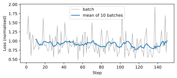
The mean loss falls a little after the first 50 steps, and the mean of 10 batches still moves up and down. In 150 steps the network learns little. The sections below show how to evaluate a model and derive SINR from its predictions, not what a trained model reaches.
10. Evaluate on the validation split#
The validation scene, Amsterdam in the sample, is not in the training split. The test split, Berlin in the sample, stays untouched for a final evaluation. The network is fully convolutional, so it predicts each validation transmitter on its full map, one per batch. The error is in dB over covered cells. As a reference, predicting the mean path gain of the training crops everywhere gives the error of a model that has learned nothing.
validation = splits["validation"]
first_map = validation.index["radio_map_id"][0].as_py()
squared, squared_mean, cells, per_transmitter = 0.0, 0.0, 0, []
predictions, references, positions = {}, {}, {}

model.eval()
start = time.perf_counter()
with torch.no_grad():
    for batch in DataLoader(validation, batch_size=1, num_workers=WORKERS):
        predicted = model(normalise(batch)) * target_std + target_mean
        mask = batch["coverage"]
        truth = batch["path_gain_db"][mask]
        error = predicted[mask] - truth
        squared += error.pow(2).sum().item()
        squared_mean += (truth - target_mean).pow(2).sum().item()
        cells += int(mask.sum())
        if mask.any():  # a transmitter without covered cells has no error
            per_transmitter.append(error.pow(2).mean().sqrt().item())
        if batch["radio_map_id"][0] == first_map:  # kept for the figures
            transmitter = int(batch["transmitter"])
            predictions[transmitter] = predicted[0, 0]
            references[transmitter] = missing(batch["path_gain_db"][0, 0], mask[0, 0])
            positions[transmitter] = batch["tx_position_m"][0]
print(f"{len(validation)} transmitters, {cells:,} covered cells, {time.perf_counter() - start:.0f} s")
print(f"RMSE: network {np.sqrt(squared / cells):.1f} dB, mean of the training crops {np.sqrt(squared_mean / cells):.1f} dB, "
      f"{np.sqrt(squared_mean / cells) - np.sqrt(squared / cells):.1f} dB higher")
print(f"RMSE per transmitter: {np.min(per_transmitter):.1f} to {np.max(per_transmitter):.1f} dB, median {np.median(per_transmitter):.1f} dB")
24 transmitters, 10,433,528 covered cells, 28 s
RMSE: network 23.5 dB, mean of the training crops 26.9 dB, 3.4 dB higher
RMSE per transmitter: 19.7 to 28.5 dB, median 23.2 dB
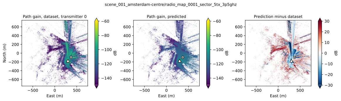
After 150 steps, the network’s error on the validation transmitters is a few dB below that of the constant training mean.
One validation transmitter: the path gain in the dataset, the prediction on the same cells, and their difference.
shown = 0
reference = references[shown]
predicted = missing(predictions[shown], ~reference.isnan())
fig, axes = plt.subplots(1, 3, figsize=(12, 3.6), constrained_layout=True)
show(axes[0], reference, f"Path gain, dataset, transmitter {shown}", "dB", extend="both", cmap="viridis", vmin=-150, vmax=-60)
show(axes[1], predicted, "Path gain, predicted", "dB", extend="both", cmap="viridis", vmin=-150, vmax=-60)
show(axes[2], predicted - reference, "Prediction minus dataset", "dB", extend="both", cmap="RdBu_r", vmin=-30, vmax=30)
for ax in axes:
    mark_transmitters(ax, positions[shown], [shown])
axes[0].set_ylabel("North (m)")
fig.suptitle(first_map, fontsize=10)
plt.show()
11. SINR and the serving transmitter from predictions#
A model of one transmitter’s path gain is enough for the quantities that involve several transmitters. RSS is the transmit power times the path gain. SINR and the serving transmitter are functions of the path gains of all transmitters of a radio map, their transmit powers and the noise power, which the index records as tx_power_w and noise_power_w. load_radio_map derives:
the RSS of transmitter i:
tx_power_w[i] * path_gain[i];the SINR of transmitter i: its RSS over the sum of the other transmitters’ RSS plus
noise_power_w;the serving transmitter: the largest value under
association_metric, the first on a tie, and -1 where no transmitter has a positive value.
The function below applies the same formulas to path gains in dB, with -inf where there is no path. Applied to the dataset’s path gain, it reproduces the dataset’s serving transmitter, and its SINR to within float32 rounding. The SINR differs slightly because load_radio_map rounds the RSS to float32 before the SINR, as the engines do; the function keeps it in float64.
def derive(path_gain_db, power_w, noise_power_w, metric):
    # RSS (W), SINR and the serving transmitter of path gains in dB, shape (T, H, W).
    gain = torch.pow(10.0, path_gain_db.double() / 10.0)  # -inf gives 0
    rss = power_w.view(-1, 1, 1) * gain
    sinr = torch.stack([rss[i] / (rss[:i].sum(0) + rss[i + 1 :].sum(0) + noise_power_w) for i in range(len(rss))])
    values = {"path_gain": gain, "rss": rss, "sinr": sinr}[metric]
    serving = values.argmax(0).masked_fill(~(values > 0).any(0), -1)
    return rss, sinr, serving


position = radio_maps.index["radio_map_id"].to_pylist().index(first_map)
row = radio_maps.index.slice(position, 1).to_pylist()[0]
whole = radio_maps[position]
power_w = torch.tensor(row["tx_power_w"], dtype=torch.float64)

stored_db = whole["path_gain_db"].masked_fill(~whole["coverage"], -torch.inf)
_, sinr, serving = derive(stored_db, power_w, row["noise_power_w"], row["association_metric"])
difference = (10 * torch.log10(sinr) - whole["sinr_db"])[whole["coverage"]].abs().max()
print(f"{first_map}: {row['n_tx']} transmitters, serving transmitter by {row['association_metric']}")
print(f"From the dataset's path gain: serving transmitter equal in {(serving == whole['serving_tx']).double().mean():.4%} of cells, "
      f"SINR within {difference:.1e} dB")
scene_001_amsterdam-centre/radio_map_0001_sector_5tx_3p5ghz: 5 transmitters, serving transmitter by sinr
From the dataset's path gain: serving transmitter equal in 100.0000% of cells, SINR within 3.2e-05 dB
The same derivation from the predicted path gains. The network predicts every cell, so the comparison keeps the cells that some transmitter serves in the dataset.
predicted_db = torch.stack([predictions[i] for i in range(row["n_tx"])])
_, predicted_sinr, predicted_serving = derive(predicted_db, power_w, row["noise_power_w"], row["association_metric"])
served = whole["serving_tx"] >= 0
best_sinr = torch.where(whole["coverage"], whole["sinr_db"], -torch.inf).amax(0)
predicted_best = 10 * torch.log10(predicted_sinr.amax(0)).float()
agreement = (predicted_serving == whole["serving_tx"])[served].double().mean()
print(f"Serving transmitter equal in {agreement:.1%} of the {int(served.sum()):,} served cells")
print(f"Best SINR on served cells: median {best_sinr[served].median():.1f} dB in the dataset, {predicted_best[served].median():.1f} dB predicted, "
      f"RMSE {(predicted_best - best_sinr)[served].pow(2).mean().sqrt():.1f} dB")

fig, axes = plt.subplots(1, 4, figsize=(15, 3.6), constrained_layout=True)
show(axes[0], missing(whole["serving_tx"], served), "Serving transmitter, dataset", "transmitter", **categories(row["n_tx"]))
show(axes[1], missing(predicted_serving, served), "Serving transmitter, predicted", "transmitter", **categories(row["n_tx"]))
show(axes[2], missing(best_sinr, served), "Best SINR, dataset", "dB", extend="both", cmap="magma", vmin=-10, vmax=40)
show(axes[3], missing(predicted_best, served), "Best SINR, predicted", "dB", extend="both", cmap="magma", vmin=-10, vmax=40)
for ax in axes:
    mark_transmitters(ax, whole["tx_position_m"])
axes[0].set_ylabel("North (m)")
plt.show()
Serving transmitter equal in 55.0% of the 1,275,052 served cells
Best SINR on served cells: median 21.1 dB in the dataset, 2.0 dB predicted, RMSE 26.7 dB
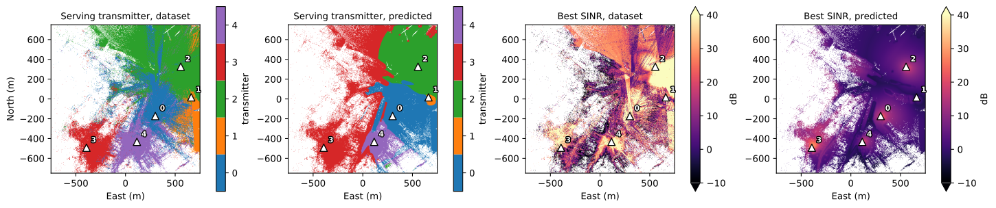
The predicted serving transmitter matches the dataset in 55% of the served cells, and the best predicted SINR has a median of 2 dB, against 21 dB in the dataset. The derivation is exact, as the check on the stored path gain shows, so the gap is the model’s: after 150 steps its path gains do not separate the transmitters as Sionna’s do.
Notes#
Normalisation. The dataset returns physical units. The statistics above come from the training split and are applied unchanged to the validation split; keep them with the model.
Randomness.
torch.manual_seedbefore the model fixes the initial weights, and the loader’sgeneratorfixes the shuffle order and the seeds of the workers, and so the crop windows whenWORKERS > 0. Without workers the crops followtorch.manual_seed. The timings, and the last digit of the loss and error values, depend on the machine.GPU. Move the model,
input_meanandinput_stdwith.to(device), and each tensor of a batch beforenormalise. The dataset itself stays on the CPU.