
Viewing the radio maps of an OWRT-RF package#
An OWRT-RF package holds Sionna RT radio maps of real city districts: for each radio map, the path gain of every transmitter on a regular grid of receivers, the scene it was solved in, and the records that say how. This tutorial opens the sample package and finds radio maps with its Parquet index. It loads one radio map and plots its path gain, the received power (RSS), the signal-to-interference-plus-noise ratio (SINR) and the serving transmitter. It draws the building footprints over the RSS and the serving transmitter. It then shows the scene inputs on the same grid, views the scene in Sionna’s 3D viewer, reads the provenance, and solves the radio map again with Sionna. Last, it compares the radio map with the same radio map on flat ground.
Outline
Setup
What a package contains
Find radio maps with the index
Load a radio map
Path gain, RSS, SINR and the serving transmitter
Building footprints as vector outlines
Scene inputs on the radio grid
The scene in 3D
Provenance
Solve the radio map again
Buildings on flat ground
The closing notes give the array conventions, the stored precision and other ways to read a package.
1. Setup#
Sections 2 to 7 need NumPy, pyarrow, pandas and Matplotlib; sections 8 and 10 need Sionna RT. Install the package with the notebook extras:
python -m pip install -e ".[rt,tutorial]"
ROOT is a package directory with its scene archives extracted into it. A package is a release of radio maps, or the output of owrt dataset package on a dataset you generated (see Packaging for release in the dataset guide). [Download location of the OWRT-RF sample package: to be added when it is published.] Check and extract a package once, inside the package directory:
sha256sum -c SHA256SUMS
for archive in scenes/*.tar.zst; do tar --zstd -xf "$archive"; done
GNU tar before 1.31 takes -I zstd instead of --zstd. The sample package takes about 0.54 GB as archives and about 1.1 GB more once extracted. The environment variable OWRT_RF_ROOT overrides the default location below. A relative location is relative to the kernel’s working directory, which Jupyter sets to the notebook’s folder. The default is therefore data/owrt-rf-sample next to the notebook, examples/data/owrt-rf-sample in the repository. Section 11 also opens the flat sample package, owrt-rf-sample-flat, from OWRT_RF_FLAT_ROOT (default data/owrt-rf-sample-flat). It takes about 0.35 GB as archives and about 1.0 GB more once extracted.
The stored outputs come from the two sample packages: six scenes with four radio maps each, computed on a GPU, and read here on a CPU. On the machine that produced them, two 16-core CPUs with 64 hardware threads, sections 8 and 10 took about 95 seconds together and the other sections about 50 seconds. Section 10 needs about 2 GB of memory on a CPU. The figures are stored as SVG: outlines, markers and text are vectors, and the radio maps are embedded with one pixel per cell, so they stay sharp when zoomed. To keep the notebook small, the whole-scene panels show every third cell in each direction, and the eight path-gain panels of section 5 every fifth; each pixel is centred on the cell it shows. The zoomed panels of section 6 show every cell. Section 3 prints the OpenWorld Radio Twin version that read the package, and section 8 the Sionna RT version.
# SVG figures: lines, markers and text stay vectors; imshow(interpolation="none") embeds one pixel per cell.
%config InlineBackend.figure_formats = ["svg"]

import hashlib
import json
import math
import os
from pathlib import Path

import matplotlib.pyplot as plt
import numpy as np
import pandas as pd
import pyarrow.compute as pc
from matplotlib import patheffects
from matplotlib.collections import LineCollection
from matplotlib.colors import ListedColormap
from matplotlib.patches import Patch, Rectangle

import openworld_radio_twin
from openworld_radio_twin import rt as owrt
from openworld_radio_twin.dataset import load_radio_map, read_index

# An OWRT-RF package with its scene archives extracted into it.
ROOT = Path(os.environ.get("OWRT_RF_ROOT", "data/owrt-rf-sample"))
if not (ROOT / "index.parquet").is_file():
    raise FileNotFoundError(f"No OWRT-RF package in {ROOT}; set OWRT_RF_ROOT to an extracted package directory")
not_extracted = [scene for scene in json.loads((ROOT / "splits.json").read_text(encoding="utf-8"))["assignment"]
                 if not (ROOT / scene).is_dir()]
if not_extracted:
    raise FileNotFoundError(f"Scene archives not extracted in {ROOT}: {', '.join(not_extracted)}; see the Setup section")
DEVICE = "auto"  # "auto" | "cuda" | "cpu": the Mitsuba variant of sections 8 and 10

PATH_GAIN_LIMITS_DB = (-150.0, -60.0)
RSS_LIMITS_DBM = (-120.0, -30.0)
SINR_LIMITS_DB = (-20.0, 60.0)
NO_DATA = "#e6e8eb"  # background shown where no transmitter reaches a cell
OVERVIEW_STEP = 3  # whole-scene panels show every third cell in each direction, to keep the notebook small
PATH_GAIN_STEP = 5  # the eight path-gain panels of section 5 show every fifth cell

pd.set_option("display.width", 160)
pd.set_option("display.max_colwidth", 80)
2. What a package contains#
A package directory holds one compressed archive per scene under scenes/ and the files that describe the package. Extraction adds one directory per scene next to them.
for path in sorted(ROOT.iterdir()):
    if path.is_dir():
        print(f"{path.name + '/':<40}{sum(1 for _ in path.iterdir()):>5} entries")
    else:
        print(f"{path.name:<40}{path.stat().st_size:>12,} bytes")
LICENSE.md                                     6,180 bytes
README.md                                      3,282 bytes
SHA256SUMS                                     1,067 bytes
dataset_manifest.json                         59,131 bytes
index.parquet                                 29,780 bytes
scene_001_amsterdam-centre/                11 entries
scene_002_berlin-potsdamer-platz/          11 entries
scene_003_paris-champ-de-mars/             11 entries
scene_004_san-francisco-embarcadero/       11 entries
scene_005_hong-kong-mid-levels/            11 entries
scene_006_bergen-bryggen/                  11 entries
scenes/                                     6 entries
splits.json                                    1,505 bytes
File |
Contents |
|---|---|
|
The layout, the snapshot the package was made from, the scenes and radio maps per split, and what was left out |
|
The request that generated the dataset, the seed derivation, the array conventions and the counts |
|
The licences and credits of the data sources of the packaged scenes |
|
The train, validation and test split of each scene |
|
One row per radio map, used in section 3 |
|
The SHA-256 checksum of every other file |
The README opens with the snapshot the package was made from:
readme = (ROOT / "README.md").read_text(encoding="utf-8")
print(readme.split("\n\n")[1])
Package of the OpenWorld Radio Twin dataset `owrt-rf-sample`, dataset format 2, generated with version 0.3.0. The manifest status is `completed`. The package is a snapshot of the dataset at index revision 1, whose `dataset_manifest.json` has the SHA-256 checksum `1d44ba7a72766339c2dcca3a310ffe3820eed3fa14ea6a140c7064a1316acf66`.
Scenes, not radio maps, are assigned to splits, because the radio maps of a scene share its geometry. Scenes whose squares overlap, or that carry the same site, form one group and share a split.
splits = json.loads((ROOT / "splits.json").read_text(encoding="utf-8"))
print(f"Fractions {splits['fractions']}, shuffled with seed {splits['seed']}")
pd.Series(splits["assignment"], name="split").rename_axis("scene").to_frame()
Fractions {'train': 0.8, 'validation': 0.1, 'test': 0.1}, shuffled with seed 0
| split | |
|---|---|
| scene | |
| scene_001_amsterdam-centre | validation |
| scene_002_berlin-potsdamer-platz | test |
| scene_003_paris-champ-de-mars | train |
| scene_004_san-francisco-embarcadero | train |
| scene_005_hong-kong-mid-levels | train |
| scene_006_bergen-bryggen | train |
LICENSE.md states the licence the package is offered under and credits every source, with the scenes that use it.
licence = (ROOT / "LICENSE.md").read_text(encoding="utf-8")
print("\n\n".join(licence.split("\n\n")[1:3]), "\n")
print("Sources:")
for line in licence.splitlines():
    if line.startswith("### "):
        print("  " + line.removeprefix("### "))
Contains information from Overture Maps Foundation and © OpenStreetMap contributors, made available under the Open Database License (ODbL) 1.0 (https://opendatacommons.org/licenses/odbl/1-0/).

This dataset is a derivative database of those data and is offered under the ODbL 1.0. Its radio arrays and images are produced from that database. The other sources below are credited as their publishers require.

Sources:
  Buildings: 3DBAG
  Terrain: Mapzen Terrain Tiles
  Surfaces: Overture Maps
  Surfaces: ESA WorldCover, via Overture Maps
  Surfaces: OpenStreetMap, via Overture Maps
  Surfaces: TomTom, via Overture Maps
  Buildings: Berlin LoD2
  Buildings: Overture Maps
  Buildings: Microsoft ML Buildings, via Overture Maps
  Buildings: OpenStreetMap, via Overture Maps
  Buildings: USGS Lidar, via Overture Maps
  Terrain: USGS 3DEP
  Buildings: doi:10.5281/zenodo.8174931, via Overture Maps
sha256sum -c SHA256SUMS checks the files from a shell. The same check in Python:
def sha256(path):
    digest = hashlib.sha256()
    with path.open("rb") as handle:
        for block in iter(lambda: handle.read(1 << 20), b""):
            digest.update(block)
    return digest.hexdigest()


checks = [line.split(maxsplit=1) for line in (ROOT / "SHA256SUMS").read_text(encoding="utf-8").splitlines()]
failed = [name for expected, name in checks if sha256(ROOT / name) != expected]
print(f"{len(checks) - len(failed)} of {len(checks)} files match SHA256SUMS; mismatches: {failed or 'none'}")
11 of 11 files match SHA256SUMS; mismatches: none
3. Find radio maps with the index#
read_index returns index.parquet as a pyarrow.Table and refuses an index built for another revision of the manifest. Each row repeats a few scene values, so radio maps can be selected without opening their records. The Parquet footer records the dataset format and the versions that wrote it; the last line is the installed version that reads it.
index = read_index(ROOT)
print(f"{index.num_rows} radio maps, {index.num_columns} columns")
for key, value in index.schema.metadata.items():
    print(f"  {key.decode()}: {value.decode()}")
print(f"Read with openworld_radio_twin {openworld_radio_twin.__version__}")

table = index.to_pandas()
table.groupby("scene", sort=False).agg(
    label=("label", "first"),
    split=("split", "first"),
    radio_maps=("name", "size"),
    tx_per_map=("n_tx", list),
    buildings=("building_source", "first"),
    terrain=("terrain_provider", "first"),
)
24 radio maps, 42 columns
  owrt.schema_version: 2
  owrt.index_revision: 1
  owrt.openworld_radio_twin_version: 0.3.0
  owrt.pyarrow_version: 25.0.0
  owrt.source_manifest_sha256: 1d44ba7a72766339c2dcca3a310ffe3820eed3fa14ea6a140c7064a1316acf66
Read with openworld_radio_twin 0.3.0
| label | split | radio_maps | tx_per_map | buildings | terrain | |
|---|---|---|---|---|---|---|
| scene | ||||||
| scene_001_amsterdam-centre | Amsterdam centre | validation | 4 | [5, 6, 8, 5] | 3dbag | Mapzen Terrain Tiles |
| scene_002_berlin-potsdamer-platz | Berlin Potsdamer Platz | test | 4 | [8, 7, 5, 8] | berlin | Mapzen Terrain Tiles |
| scene_003_paris-champ-de-mars | Paris Champ de Mars | train | 4 | [7, 5, 6, 8] | global | Mapzen Terrain Tiles |
| scene_004_san-francisco-embarcadero | San Francisco Embarcadero | train | 4 | [5, 7, 4, 8] | global | USGS 3DEP |
| scene_005_hong-kong-mid-levels | Hong Kong Mid-Levels | train | 4 | [4, 7, 8, 8] | global | Mapzen Terrain Tiles |
| scene_006_bergen-bryggen | Bergen Bryggen | train | 4 | [7, 6, 5, 8] | global | Mapzen Terrain Tiles |
The radio settings are the same in every radio map of the sample:
shared = ["engine", "frequency_hz", "bandwidth_hz", "resolution_m", "rows", "columns", "receiver_height_m", "samples_per_tx", "max_depth", "association_metric"]
print(table[shared].drop_duplicates().T.to_string(header=False))
engine                    sionna
frequency_hz        3500000000.0
bandwidth_hz           1000000.0
resolution_m                 1.0
rows                        1500
columns                     1500
receiver_height_m            1.5
samples_per_tx         100000000
max_depth                      8
association_metric          sinr
A selection is a filter on the columns. With pyarrow, the radio maps of one city with eight transmitters. The values match one radio map of the sample package; change them for another package.
selected = index.filter((pc.field("site") == "amsterdam") & (pc.field("n_tx") == 8))
selected.select(["radio_map_id", "split", "n_tx", "seed"]).to_pandas()
| radio_map_id | split | n_tx | seed | |
|---|---|---|---|---|
| 0 | scene_001_amsterdam-centre/radio_map_0003_sector_8tx_3p5ghz | validation | 8 | 3124613955 |
The same kind of selection with pandas: training radio maps with at least seven transmitters. Any Parquet reader opens the file; only read_index checks its revision.
table.query("split == 'train' and n_tx >= 7")[["radio_map_id", "n_tx", "building_source", "terrain_provider"]]
| radio_map_id | n_tx | building_source | terrain_provider | |
|---|---|---|---|---|
| 8 | scene_003_paris-champ-de-mars/radio_map_0001_sector_7tx_3p5ghz | 7 | global | Mapzen Terrain Tiles |
| 11 | scene_003_paris-champ-de-mars/radio_map_0004_sector_8tx_3p5ghz | 8 | global | Mapzen Terrain Tiles |
| 13 | scene_004_san-francisco-embarcadero/radio_map_0002_sector_7tx_3p5ghz | 7 | global | USGS 3DEP |
| 15 | scene_004_san-francisco-embarcadero/radio_map_0004_sector_8tx_3p5ghz | 8 | global | USGS 3DEP |
| 17 | scene_005_hong-kong-mid-levels/radio_map_0002_sector_7tx_3p5ghz | 7 | global | Mapzen Terrain Tiles |
| 18 | scene_005_hong-kong-mid-levels/radio_map_0003_sector_8tx_3p5ghz | 8 | global | Mapzen Terrain Tiles |
| 19 | scene_005_hong-kong-mid-levels/radio_map_0004_sector_8tx_3p5ghz | 8 | global | Mapzen Terrain Tiles |
| 20 | scene_006_bergen-bryggen/radio_map_0001_sector_7tx_3p5ghz | 7 | global | Mapzen Terrain Tiles |
| 23 | scene_006_bergen-bryggen/radio_map_0004_sector_8tx_3p5ghz | 8 | global | Mapzen Terrain Tiles |
4. Load a radio map#
The paths in the index are relative to the package directory. load_radio_map reads a radio map’s record and its stored path gain, and derives RSS, SINR and the serving transmitter from the transmit powers and the noise power the record keeps. The arrays are linear; path_gain_db, rss_dbm and sinr_db give them in dB and dBm, with -inf where the transmitter contributes nothing to the cell (stored path gain 0).
row = (selected if selected.num_rows else index).to_pylist()[0]  # the first radio map if nothing matches
radio_map = load_radio_map(ROOT / row["record"])
record = radio_map.record
print(row["radio_map_id"])
for name in ("path_gain", "rss", "sinr", "association"):
    array = getattr(radio_map, name)
    print(f"  {name:<12}{str(array.dtype):<9}{array.shape}")
scene_001_amsterdam-centre/radio_map_0003_sector_8tx_3p5ghz
  path_gain   float32  (8, 1500, 1500)
  rss         float32  (8, 1500, 1500)
  sinr        float32  (8, 1500, 1500)
  association int32    (1500, 1500)
The arrays run south to north in their rows and west to east in their columns. grid places them in the scene frame: metres east and north of the scene centre, with the first sample at the centre of the south-west cell.
grid = radio_map.grid
n_tx, rows, columns = radio_map.path_gain.shape
print(f"First sample at east {grid.first_sample_east_m} m, north {grid.first_sample_north_m} m")
print(f"Cell steps {grid.column_step_m} m east, {grid.row_step_m} m north")

# The edges of the grid, for imshow(origin="lower"): row 0 at the bottom (south).
EXTENT = (
    grid.first_sample_east_m - grid.column_step_m / 2,
    grid.first_sample_east_m + (columns - 0.5) * grid.column_step_m,
    grid.first_sample_north_m - grid.row_step_m / 2,
    grid.first_sample_north_m + (rows - 0.5) * grid.row_step_m,
)
TX_POSITIONS = np.asarray(record["radio"]["tx_positions_enu_m"])  # where the engine placed them

pd.DataFrame(
    {
        "east (m)": TX_POSITIONS[:, 0],
        "north (m)": TX_POSITIONS[:, 1],
        "height above ground (m)": row["tx_height_agl_m"],
        "power (dBm)": row["tx_power_dbm"],
        "azimuth (deg)": row["tx_azimuth_deg"],
        "downtilt (deg)": row["tx_downtilt_deg"],
    }
).round(1).rename_axis("transmitter")
First sample at east -749.5 m, north -749.5 m
Cell steps 1.0 m east, 1.0 m north
| east (m) | north (m) | height above ground (m) | power (dBm) | azimuth (deg) | downtilt (deg) | |
|---|---|---|---|---|---|---|
| transmitter | ||||||
| 0 | -4.3 | 4.0 | 27.9 | 35.3 | 346.0 | 11.5 |
| 1 | 233.8 | -190.3 | 20.6 | 28.7 | 293.3 | 1.9 |
| 2 | 250.9 | -384.6 | 31.6 | 34.3 | 245.5 | 3.6 |
| 3 | -581.9 | 26.3 | 30.0 | 32.2 | 272.2 | 11.9 |
| 4 | -469.2 | 183.9 | 26.2 | 27.7 | 181.4 | 1.4 |
| 5 | -31.0 | 428.2 | 17.0 | 35.3 | 231.3 | 9.9 |
| 6 | 274.8 | 106.5 | 22.3 | 32.2 | 12.2 | 3.0 |
| 7 | -211.9 | 260.4 | 17.2 | 28.5 | 348.7 | 4.1 |
5. Path gain, RSS, SINR and the serving transmitter#
Two small helpers draw an array of the radio grid in scene metres and mark the transmitters. Cells with no contribution from a transmitter are left out and show the grey background. The colour scales have fixed limits. Values beyond a limit take the end colour, and an arrow on the colour bar marks the side where values are cut.
def finite(values):
    # -inf (no contribution to the cell) becomes NaN, which imshow leaves transparent.
    return np.where(np.isfinite(values), values, np.nan)


def show(ax, image, title, label=None, extent=EXTENT, step=1, extend="neither", **style):
    # step > 1 draws every step-th cell in each direction, each pixel centred on the cell it shows.
    first = step // 2
    cells = image[first::step, first::step]
    west, east, south, north = extent
    width, height = (east - west) / image.shape[1], (north - south) / image.shape[0]
    west, south = west + (first - (step - 1) / 2) * width, south + (first - (step - 1) / 2) * height
    extent = (west, west + cells.shape[1] * step * width, south, south + cells.shape[0] * step * height)
    ax.set_facecolor(NO_DATA)
    shown = ax.imshow(cells, origin="lower", extent=extent, interpolation="none", **style)
    ax.set_title(title)
    if label is not None:
        ax.figure.colorbar(shown, ax=ax, label=label, shrink=0.8, extend=extend)
    return shown


def transmitter_colours(count):
    # tab10 without its grey, which would look like the no-data background; turbo for more than nine.
    colours = [colour for i, colour in enumerate(plt.cm.tab10.colors) if i != 7]
    return ListedColormap(colours[:count] if count <= len(colours) else plt.cm.turbo(np.linspace(0, 1, count)))


OUTLINE = [patheffects.withStroke(linewidth=2.5, foreground="black")]


def mark_transmitters(ax, which=None):
    # Call it after the axes limits are set: near their east or north edge the label goes to the other side.
    west, east_limit = ax.get_xlim()
    south, north_limit = ax.get_ylim()
    for number in range(n_tx) if which is None else [which]:
        east, north, _ = TX_POSITIONS[number]
        ax.plot(east, north, "^", color="white", markeredgecolor="black", markersize=7)
        right = east < east_limit - 0.04 * (east_limit - west)
        up = north < north_limit - 0.03 * (north_limit - south)
        ax.annotate(str(number), (east, north), xytext=(4 if right else -4, 4 if up else -4), textcoords="offset points",
                    ha="left" if right else "right", va="bottom" if up else "top",
                    color="white", fontsize=8, fontweight="bold", path_effects=OUTLINE)
The path gain of each transmitter, on one colour scale. It depends on the environment and the antenna, not on the transmit power.
gain_db = radio_map.path_gain_db
panel_rows = math.ceil(n_tx / 4)
fig, axes = plt.subplots(panel_rows, 4, figsize=(13, 3.2 * panel_rows), sharex=True, sharey=True, squeeze=False,
                         constrained_layout=True)
for number, ax in enumerate(axes.flat):
    if number >= n_tx:
        ax.set_visible(False)
        continue
    image = show(ax, finite(gain_db[number]), f"Transmitter {number}", step=PATH_GAIN_STEP, cmap="viridis",
                 vmin=PATH_GAIN_LIMITS_DB[0], vmax=PATH_GAIN_LIMITS_DB[1])
    mark_transmitters(ax, number)
for ax in axes[:, 0]:
    ax.set_ylabel("North (m)")
for ax in axes[-1]:
    ax.set_xlabel("East (m)")
fig.colorbar(image, ax=axes, label="Path gain (dB)", shrink=0.8, extend="min")
plt.show()

positive = gain_db[np.isfinite(gain_db)]
print(f"Positive path gains below {PATH_GAIN_LIMITS_DB[0]:g} dB: {(positive < PATH_GAIN_LIMITS_DB[0]).mean():.1%}")
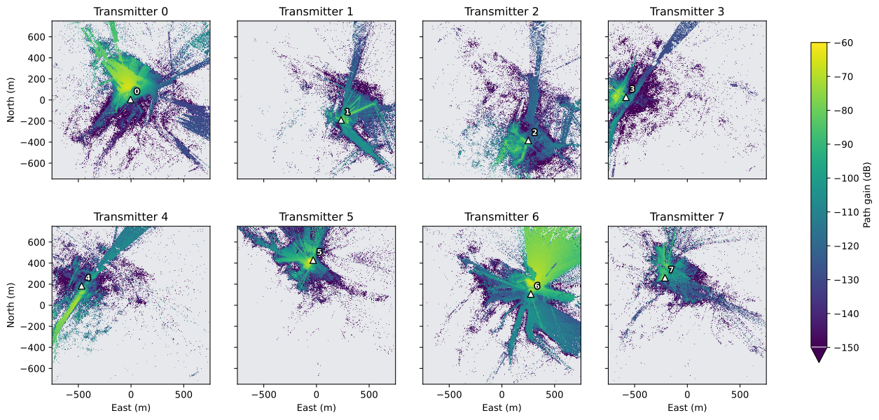
Positive path gains below -150 dB: 20.9%
Across transmitters, per cell: the strongest RSS, the SINR of the serving transmitter, and the serving transmitter itself. The record’s association_metric is SINR, so the serving transmitter is the one with the highest SINR, and -1 where no transmitter reaches the cell. With this metric, the SINR of the serving transmitter is also the highest SINR over the transmitters in each cell.
best_rss_dbm = finite(radio_map.rss_dbm.max(axis=0))
serving_sinr_db = np.take_along_axis(radio_map.sinr_db, np.maximum(radio_map.association, 0)[None], axis=0)[0]
serving_sinr_db = np.where(radio_map.association >= 0, finite(serving_sinr_db), np.nan)
serving = np.where(radio_map.association >= 0, radio_map.association, np.nan)
TX_COLOURS = transmitter_colours(n_tx)
RSS_STYLE = dict(cmap="inferno", vmin=RSS_LIMITS_DBM[0], vmax=RSS_LIMITS_DBM[1])
SERVING_STYLE = dict(cmap=TX_COLOURS, vmin=-0.5, vmax=n_tx - 0.5)

fig, axes = plt.subplots(1, 3, figsize=(15, 4.6), sharey=True, constrained_layout=True)
show(axes[0], best_rss_dbm, "Strongest RSS", "RSS (dBm)", step=OVERVIEW_STEP, extend="min", **RSS_STYLE)
show(axes[1], serving_sinr_db, "SINR of the serving transmitter", "SINR (dB)", step=OVERVIEW_STEP, extend="both",
     cmap="magma", vmin=SINR_LIMITS_DB[0], vmax=SINR_LIMITS_DB[1])
show(axes[2], serving, "Serving transmitter", "transmitter", step=OVERVIEW_STEP, **SERVING_STYLE)
axes[0].set_ylabel("North (m)")
for ax in axes:
    ax.set_xlabel("East (m)")
    mark_transmitters(ax)
plt.show()

served = radio_map.association >= 0
print(f"Cells reached by at least one transmitter: {served.mean():.1%}")
print(f"Median over those cells: strongest RSS {np.nanmedian(best_rss_dbm):.1f} dBm, SINR {np.nanmedian(serving_sinr_db):.1f} dB")
print(f"Beyond the colour limits: RSS below {RSS_LIMITS_DBM[0]:g} dBm {(best_rss_dbm[served] < RSS_LIMITS_DBM[0]).mean():.1%}, "
      f"SINR below {SINR_LIMITS_DB[0]:g} dB {(serving_sinr_db[served] < SINR_LIMITS_DB[0]).mean():.1%} "
      f"and above {SINR_LIMITS_DB[1]:g} dB {(serving_sinr_db[served] > SINR_LIMITS_DB[1]).mean():.1%} of those cells")
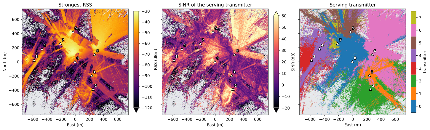
Cells reached by at least one transmitter: 79.2%
Median over those cells: strongest RSS -77.4 dBm, SINR 18.7 dB
Beyond the colour limits: RSS below -120 dBm 8.5%, SINR below -20 dB 3.7% and above 60 dB 7.6% of those cells
6. Building footprints as vector outlines#
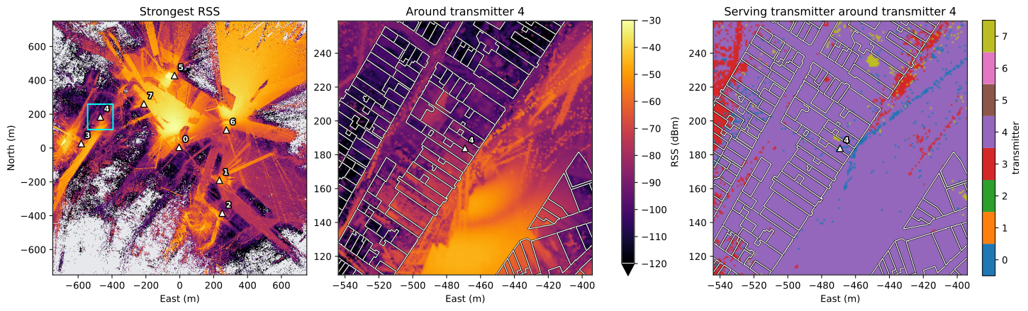
provenance.json in the scene directory keeps the footprint of every building of the scene in scene metres under local_buildings: the footprints of the building source, in source_buildings.json, converted to the scene frame. Drawn as vector lines they stay sharp at any zoom, and they line up with the radio grid because both use the same frame.
scene_dir = ROOT / row["scene"]
provenance = json.loads((scene_dir / "provenance.json").read_text(encoding="utf-8"))
footprints = [
    np.asarray(ring)[:, :2]
    for building in provenance["local_buildings"]
    for ring in (building["exterior"], *building["holes"])
]
print(f"{len(provenance['local_buildings'])} buildings, {len(footprints)} outline rings, {sum(map(len, footprints)):,} vertices")


def draw_buildings(ax, rings, linewidth):
    # A black edge keeps the white outlines visible on bright cells.
    effects = [patheffects.withStroke(linewidth=2 * linewidth, foreground="black")]
    ax.add_collection(LineCollection(rings, colors="white", linewidths=linewidth, path_effects=effects))


def rings_in(window):
    # The rings whose bounding box overlaps window (west, east, south, north).
    west, east, south, north = window
    return [ring for ring in footprints
            if ring[:, 0].max() >= west and ring[:, 0].min() <= east and ring[:, 1].max() >= south and ring[:, 1].min() <= north]
4121 buildings, 4918 outline rings, 75,417 vertices
The whole scene with the position of the window, and a window of 150 by 150 cells around the transmitter with the most outline vertices near it. The window draws every cell, so the single cells are visible next to the outlines.
HALF = min(75, rows // 2, columns // 2)  # cells on each side of the transmitter
vertices = np.concatenate(footprints)
near = [int((np.abs(vertices - TX_POSITIONS[number, :2]) <= HALF * grid.column_step_m).all(axis=1).sum()) for number in range(n_tx)]
focus = int(np.argmax(near))
east, north, _ = TX_POSITIONS[focus]
# The window's first row and column, kept inside the grid.
first_column = int(np.clip(round((east - EXTENT[0]) / grid.column_step_m) - HALF, 0, columns - 2 * HALF))
first_row = int(np.clip(round((north - EXTENT[2]) / grid.row_step_m) - HALF, 0, rows - 2 * HALF))
cells = np.s_[first_row:first_row + 2 * HALF, first_column:first_column + 2 * HALF]
window = (
    EXTENT[0] + first_column * grid.column_step_m,
    EXTENT[0] + (first_column + 2 * HALF) * grid.column_step_m,
    EXTENT[2] + first_row * grid.row_step_m,
    EXTENT[2] + (first_row + 2 * HALF) * grid.row_step_m,
)

fig, axes = plt.subplots(1, 3, figsize=(15, 4.8), constrained_layout=True)
show(axes[0], best_rss_dbm, "Strongest RSS", step=OVERVIEW_STEP, **RSS_STYLE)
axes[0].add_patch(Rectangle(window[::2], window[1] - window[0], window[3] - window[2], fill=False, edgecolor="cyan", linewidth=1.5))
image = show(axes[1], best_rss_dbm[cells], f"Around transmitter {focus}", extent=window, **RSS_STYLE)
fig.colorbar(image, ax=axes[:2], label="RSS (dBm)", shrink=0.8, extend="min")
show(axes[2], serving[cells], f"Serving transmitter around transmitter {focus}", "transmitter", extent=window, **SERVING_STYLE)
for ax in axes[1:]:
    draw_buildings(ax, rings_in(window), 0.9)
    ax.set_xlim(window[:2])
    ax.set_ylim(window[2:])
for ax in axes:
    ax.set_xlabel("East (m)")
    mark_transmitters(ax)
axes[0].set_ylabel("North (m)")
plt.show()
7. Scene inputs on the radio grid#
A scene directory also stores the scene as arrays. Two of them sit on the cell centres of the radio grid, rows south to north:
building_rasters(named in the record’sradioblock): the roof height above ground (NaN where there is no building, so grey in the figure), the building footprint mask (the cell centre lies under a building) and the indoor mask (the receiver point lies inside a building);the measurement surface’s
.npz: the cell centres in the scene frame; their height minus the receiver height is the height of the terrain mesh under the cell centre. Heights in the scene frame are relative to the terrain at the scene centre.
The terrain arrays under terrain/ are coarser. The surface class of each terrain cell is looked up at the radio cell centres. A package of buildings on flat ground has no terrain/ directory and no surface classes; the surface class is then -1 in every cell, as in the PyTorch dataset.
scene_record = json.loads((scene_dir / "scene_info.json").read_text(encoding="utf-8"))
rasters = np.load(scene_dir / record["radio"]["building_rasters"])
surface = np.load((scene_dir / record["radio"]["measurement_surface"]).with_suffix(".npz"))
centres = surface["cell_centers_enu_m"]  # (rows, columns, 3)
ground_m = centres[..., 2] - row["receiver_height_m"]

# Surface classes are stored per terrain cell; terrain axes are cell edges in scene metres.
environment = scene_record["shared_assets"].get("environment")
if environment is None:  # buildings on flat ground
    surface_classes, class_names = np.full(centres.shape[:2], -1), {}
    print("No terrain and no surface classes")
else:
    terrain = json.loads((scene_dir / environment).read_text(encoding="utf-8"))
    classes = np.load(scene_dir / scene_record["shared_assets"]["environment_arrays"]["surface_classes"])
    terrain_rows = np.clip(np.searchsorted(terrain["north_m"], centres[:, 0, 1], side="right") - 1, 0, classes.shape[0] - 1)
    terrain_columns = np.clip(np.searchsorted(terrain["east_m"], centres[0, :, 0], side="right") - 1, 0, classes.shape[1] - 1)
    surface_classes = classes[np.ix_(terrain_rows, terrain_columns)]
    class_names = terrain["surface_classes"]  # id -> name
    print(f"Terrain cells {terrain['east_m'][1] - terrain['east_m'][0]:g} m, radio cells {grid.column_step_m:g} m")

footprint = rasters["footprint_mask"]
indoor = rasters["receiver_in_building_mask"]
roof_m = rasters["roof_height_agl_m"]
low_roof = footprint & ~indoor
print(f"Surface classes: {class_names}")
print(f"Footprint cells {footprint.mean():.1%}, indoor cells {indoor.mean():.1%}, footprint without indoor receiver {low_roof.mean():.2%}")
print(f"Footprint cells without indoor receiver whose roof is below the receiver height: {(roof_m[low_roof] < row['receiver_height_m']).mean():.0%}")
print(f"Cells reached by a transmitter: indoor {served[indoor].mean():.1%}, outdoor {served[~indoor].mean():.1%}")
Terrain cells 5 m, radio cells 1 m
Surface classes: {'0': 'ground', '1': 'vegetation', '2': 'paved', '3': 'water'}
Footprint cells 29.3%, indoor cells 28.9%, footprint without indoor receiver 0.37%
Footprint cells without indoor receiver whose roof is below the receiver height: 100%
Cells reached by a transmitter: indoor 71.4%, outdoor 82.3%
CLASS_COLOURS = {"ground": "#b08d57", "vegetation": "#5a9a4a", "paved": "#9a9a9a", "water": "#4a7fb5"}
ROOF_LIMIT_M = 40

fig, axes = plt.subplots(1, 5, figsize=(18, 3.9), sharey=True, constrained_layout=True)
show(axes[0], roof_m, "Roof height", "m above ground", step=OVERVIEW_STEP, extend="max", cmap="viridis", vmin=0, vmax=ROOF_LIMIT_M)
show(axes[1], footprint, "Building footprint", step=OVERVIEW_STEP, cmap="Greys", vmin=0, vmax=1.5)
show(axes[2], indoor, "Receiver inside a building", step=OVERVIEW_STEP, cmap="Greys", vmin=0, vmax=1.5)
show(axes[3], ground_m, "Ground elevation", "m relative to the scene centre", step=OVERVIEW_STEP, cmap="cividis")
if class_names:
    class_ids = sorted(int(key) for key in class_names)
    class_map = ListedColormap([CLASS_COLOURS.get(class_names[str(key)], "black") for key in class_ids])
    show(axes[4], surface_classes, "Surface class", step=OVERVIEW_STEP, cmap=class_map, vmin=class_ids[0] - 0.5, vmax=class_ids[-1] + 0.5)
    axes[4].legend(handles=[Patch(color=class_map(i), label=class_names[str(key)]) for i, key in enumerate(class_ids)],
                   loc="upper left", bbox_to_anchor=(1.02, 1), fontsize=8, frameon=False)
else:
    show(axes[4], np.full(surface_classes.shape, np.nan), "No surface classes", step=OVERVIEW_STEP, vmin=0, vmax=1)
axes[0].set_ylabel("North (m)")
for ax in axes:
    ax.set_xlabel("East (m)")
plt.show()

print(f"Footprint cells with a roof above {ROOF_LIMIT_M} m, in the top colour: {(roof_m[footprint] > ROOF_LIMIT_M).mean():.1%}")

Footprint cells with a roof above 40 m, in the top colour: 0.8%
The measurement surface also runs under buildings, so receivers inside a building are part of the grid. The indoor mask lets a metric or a loss include or exclude them. A footprint cell has no indoor receiver where the roof is lower than the receiver height, as the check above shows.
8. The scene in 3D#
The scene directory is a compiled Sionna scene. owrt.load_scene loads its scene.xml as a native sionna.rt.Scene and selects the Mitsuba variant from device, which is why sionna.rt is imported after it. The radio map’s transmitters are added as native Transmitters at the positions the record keeps, with the carrier, the noise bandwidth and the arrays the Sionna engine used. The engine uses one array for every transmitter of a radio map, chosen from the first transmitter’s pattern, and the record names it in engine_details.tx_array: an 8 x 2 TR 38.901 panel (8x2_tr38901) or one isotropic element (1x1_iso). Sionna’s orientation angles follow from the compass azimuth and the downtilt: alpha = 90° - azimuth, wrapped into [-180°, 180°), beta = downtilt.
scene = owrt.load_scene(scene_dir, device=DEVICE)

import mitsuba as mi  # noqa: E402
import sionna.rt as rt  # noqa: E402 - the Mitsuba variant is now fixed

scene.frequency = row["frequency_hz"]
scene.bandwidth = row["bandwidth_hz"]
if record["engine_details"]["tx_array"] == "1x1_iso":
    scene.tx_array = rt.PlanarArray(num_rows=1, num_cols=1, pattern="iso", polarization="V")
else:
    scene.tx_array = rt.PlanarArray(num_rows=8, num_cols=2, pattern="tr38901", polarization="V")
scene.rx_array = rt.PlanarArray(num_rows=1, num_cols=1, pattern="iso", polarization="V")

for number, position in enumerate(TX_POSITIONS):
    alpha = (90.0 - row["tx_azimuth_deg"][number] + 180.0) % 360.0 - 180.0
    scene.add(
        rt.Transmitter(
            name=f"tx-{number}",
            position=position.tolist(),
            orientation=[math.radians(alpha), math.radians(row["tx_downtilt_deg"][number]), 0.0],
            power_dbm=row["tx_power_dbm"][number],
        )
    )
print(f"Sionna RT {rt.__version__}, Mitsuba variant {mi.variant()}; {len(scene.transmitters)} transmitters at {scene.frequency.numpy().item() / 1e9:g} GHz")
print(f"Thermal noise power: scene {scene.thermal_noise_power.numpy().item():.4e} W, record {record['radio']['noise_power_w']:.4e} W")
Sionna RT 2.0.1, Mitsuba variant llvm_ad_mono_polarized; 8 transmitters at 3.5 GHz
Thermal noise power: scene 4.0453e-15 W, record 4.0453e-15 W
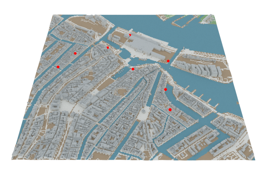
scene.preview() is Sionna’s interactive viewer: drag to orbit, scroll to zoom, right-drag to pan. Water is blue, vegetation green, bare ground brown, buildings and paved surfaces grey, and the transmitters red. JupyterLab renders it directly. VS Code must be allowed to fetch the widget’s JavaScript: add "jupyter.widgetScriptSources": ["jsdelivr.com", "unpkg.com"] to its settings, reload the window and restart the kernel. The widget lives in the running kernel, so a notebook opened without one shows no viewer here. The cell carries the tag skip-execution, so jupyter nbconvert --execute skips it when the stored outputs are regenerated; its widget state would add tens of megabytes to the file.
scene.preview(resolution=(1400, 900))
For the stored notebook, scene.render() traces the same scene from a fixed camera with Mitsuba’s path tracer, looking north over the whole scene. It returns the image as a bitmap.
camera = rt.Camera(position=[0.0, -1700.0, 1750.0], look_at=[0.0, -130.0, 0.0])
bitmap = scene.render(camera=camera, resolution=(960, 600), num_samples=64, return_bitmap=True)
pixels = np.asarray(bitmap.convert(component_format=mi.Struct.Type.UInt8, srgb_gamma=True))

fig, ax = plt.subplots(figsize=(9.6, 6), constrained_layout=True)
ax.imshow(pixels, interpolation="none")
ax.set_axis_off()
plt.show()
9. Provenance#
The scene’s scene_info.json lists the data sources of each layer with their release and licence. LICENSE.md repeats them for the whole package, with the full credit lines.
scene_provenance = scene_record["provenance"]
print(f"{scene_provenance['exported_building_count']} buildings from {scene_provenance['building_provider']}, "
      f"{scene_provenance['boundary_excluded_building_count']} crossing the scene boundary left out")
pd.DataFrame(scene_provenance["licences"])[["layer", "source", "release", "license"]]
4121 buildings from 3DBAG, 174 crossing the scene boundary left out
| layer | source | release | license | |
|---|---|---|---|---|
| 0 | buildings | 3DBAG | None | CC BY 4.0 |
| 1 | terrain | Mapzen Terrain Tiles | None | Per upstream source for the tile region |
| 2 | surfaces | Overture Maps | 2026-09-23.1 | ODbL 1.0 |
| 3 | surfaces | ESA WorldCover, via Overture Maps | 2026-09-23.1 | CC BY 4.0 |
| 4 | surfaces | OpenStreetMap, via Overture Maps | 2026-09-23.1 | ODbL 1.0 |
| 5 | surfaces | TomTom, via Overture Maps | 2026-09-23.1 | ODbL 1.0 |
The radio map’s record keeps its expanded request and what the solver did. The request holds every transmitter, the solver seed, the number of rays per transmitter, the path depth (the maximum number of interactions per path) and the propagation switches; engine_details holds the Sionna version, the device and the arrays.
request = record["request"]
details = record["engine_details"]
flags = {name: request["engine_config"][name] for name in ("los", "specular_reflection", "diffuse_reflection", "refraction", "diffraction", "edge_diffraction", "diffraction_lit_region")}
print(f"Sionna RT {details['version']}, variant {details['variant']}")
print(f"Seed {request['seed']}, {request['samples_per_tx']:,} rays per transmitter, depth {request['max_depth']}, array {details['tx_array']}")
print(f"Receivers {request['receiver_height_m']} m above ground on {request['resolution_m']:g} m cells: {details['measurement_surface']}")
print("Propagation:", ", ".join(name for name, enabled in flags.items() if enabled))
print("Disabled:   ", ", ".join(name for name, enabled in flags.items() if not enabled))
print("Warnings:")
for warning in record["warnings"]:
    print("  -", warning)
Sionna RT 2.0.1, variant cuda_ad_mono_polarized
Seed 3124613955, 100,000,000 rays per transmitter, depth 8, array 8x2_tr38901
Receivers 1.5 m above ground on 1 m cells: terrain-following triangular mesh
Propagation: los, specular_reflection, refraction, diffraction_lit_region
Disabled:    diffuse_reflection, diffraction, edge_diffraction
Warnings:
  - Global terrain uses a multi-source Mapzen mosaic; regional source accuracy, datum consistency, and attribution must be reviewed in exported metadata.
  - 1702 road sections lacked source width; deterministic class widths are recorded as assumptions.
  - 611 road sections lacked source surface; deterministic road-class surfaces are recorded as assumptions.
10. Solve the radio map again#
The record holds the solver settings, and section 8 already set up the scene from the full scene.xml. The solve therefore applies to records whose engine_details.geometry_masked is false, as in every record of the sample; the code checks it. The measurement surface is the stored .ply of the record’s radio block, loaded as a Mitsuba mesh. The solver call takes the record’s seed, number of rays per transmitter, depth and propagation switches; it is unchanged Sionna.
if details["geometry_masked"]:
    raise ValueError("this record excludes geometry classes; remove them from scene.xml first")
measurement_surface = rt.load_mesh(str(scene_dir / record["radio"]["measurement_surface"]), flip_normals=False)
resolved = rt.RadioMapSolver()(
    scene,
    measurement_surface=measurement_surface,
    samples_per_tx=request["samples_per_tx"],
    max_depth=request["max_depth"],
    seed=request["seed"],
    **flags,
)
# Reading the result makes Sionna evaluate it; the ray tracing runs here.
triangles = resolved.path_gain.numpy()
print(f"{type(resolved).__name__}: {measurement_surface.face_count():,} triangles, two per cell")
print(f"Sionna RT {rt.__version__} here, {details['version']} for the record")
MeshRadioMap: 4,500,000 triangles, two per cell
Sionna RT 2.0.1 here, 2.0.1 for the record
The measurement surface has two triangles per cell, cell by cell in row order. The dataset stores the area-weighted mean of the two triangles of each cell, so the same reduction puts the new result on the radio grid. The comparison is in dB, over the cells where both results are positive.
areas = surface["triangle_areas_m2"]  # (rows, columns, 2)
triangles = triangles.reshape(n_tx, rows, columns, 2)
path_gain = ((triangles * areas).sum(axis=-1) / areas.sum(axis=-1)).astype(np.float32)

stored = radio_map.path_gain > 0
again = path_gain > 0
both = stored & again
with np.errstate(divide="ignore"):
    difference_db = np.abs(10 * np.log10(path_gain[both]) - radio_map.path_gain_db[both])
print(f"Positive values (transmitter, cell): stored {stored.sum():,}, solved again {again.sum():,}, in both {both.sum():,}")
print(f"|difference| where both are positive: median {np.median(difference_db):.4f} dB, "
      f"99th percentile {np.percentile(difference_db, 99):.4f} dB")
print(f"Within 0.01 dB: {(difference_db <= 0.01).mean():.4%}; positive in one result only: {(stored ^ again).sum():,} values")
Positive values (transmitter, cell): stored 4,253,070, solved again 4,253,072, in both 4,252,510
|difference| where both are positive: median 0.0025 dB, 99th percentile 0.0050 dB
Within 0.01 dB: 99.8084%; positive in one result only: 1,122 values
The stored outputs of this section ran with the Sionna RT version of the record, on a CPU (the Mitsuba variant printed in section 8), while the record was solved on a GPU. With the record’s seed and settings, all but 0.2% of the values agree within 0.01 dB, twice the largest rounding error of the stored values (0.005 dB). The median and the 99th percentile match those of rounding to 0.01 dB steps. About a thousand values are positive in one result only. Solving again reproduces the radio map closely, but not bit for bit.
11. Buildings on flat ground#
A second sample package, owrt-rf-sample-flat, holds the same scenes as buildings on flat ground: no terrain, no surface classes, and concrete ground and buildings (Buildings on flat ground in the dataset guide). It was generated with the same dataset seed and scene list. Its radio maps therefore have the same transmitters as the terrain version, and the two packages pair up radio map for radio map by radio_map_id.
# The flat sample package, extracted like ROOT.
FLAT_ROOT = Path(os.environ.get("OWRT_RF_FLAT_ROOT", "data/owrt-rf-sample-flat"))
if not (FLAT_ROOT / "index.parquet").is_file():
    raise FileNotFoundError(f"No OWRT-RF package in {FLAT_ROOT}; set OWRT_RF_FLAT_ROOT to the extracted flat package")
matches = read_index(FLAT_ROOT).filter(pc.field("radio_map_id") == row["radio_map_id"]).to_pylist()
if not matches:
    raise ValueError(f"{row['radio_map_id']} is not in {FLAT_ROOT}; the two packages must come from the same scene list and dataset seed")
flat_row = matches[0]
flat_map = load_radio_map(FLAT_ROOT / flat_row["record"])
flat_positions = np.asarray(flat_map.record["radio"]["tx_positions_enu_m"])

print(row["radio_map_id"])
for name, values in (("terrain", row), ("flat", flat_row)):
    print(f"  {name:<8}terrain {values['terrain_provider']}, material profile {values['material_profile']}, seed {values['seed']}")
same = np.allclose(flat_positions[:, :2], TX_POSITIONS[:, :2]) and np.allclose(flat_row["tx_height_agl_m"], row["tx_height_agl_m"])
print(f"Same transmitter east, north and height above ground: {same}; "
      f"their up coordinates differ by up to {np.abs(flat_positions[:, 2] - TX_POSITIONS[:, 2]).max():.1f} m")

flat_rss_dbm = finite(flat_map.rss_dbm.max(axis=0))
flat_served = flat_map.association >= 0
difference_db = np.where(served & flat_served, flat_rss_dbm - best_rss_dbm, np.nan)

# The terrain version is the RSS panel of section 5.
DIFFERENCE_LIMIT_DB = 20
fig, axes = plt.subplots(1, 2, figsize=(10.5, 4.6), sharey=True, constrained_layout=True)
show(axes[0], flat_rss_dbm, "Strongest RSS, flat ground", "RSS (dBm)", step=OVERVIEW_STEP, extend="min", **RSS_STYLE)
show(axes[1], difference_db, "Flat ground minus terrain", "RSS difference (dB)", step=OVERVIEW_STEP, extend="both", cmap="RdBu_r",
     vmin=-DIFFERENCE_LIMIT_DB, vmax=DIFFERENCE_LIMIT_DB)
axes[0].set_ylabel("North (m)")
for ax in axes:
    ax.set_xlabel("East (m)")
    mark_transmitters(ax)
plt.show()

compared = np.isfinite(difference_db)
print(f"Cells reached by at least one transmitter: terrain {served.mean():.1%}, flat ground {flat_served.mean():.1%}")
print(f"Flat ground minus terrain where both are reached: median {np.median(difference_db[compared]):+.1f} dB, "
      f"more than 10 dB apart in {(np.abs(difference_db[compared]) > 10).mean():.1%} of the cells, "
      f"more than {DIFFERENCE_LIMIT_DB} dB (the end colours) in {(np.abs(difference_db[compared]) > DIFFERENCE_LIMIT_DB).mean():.1%}")
strong = compared & (best_rss_dbm >= -90)
weak = compared & (best_rss_dbm < -90)
print(f"Median |difference|: {np.median(np.abs(difference_db[strong])):.1f} dB where the terrain RSS is at least -90 dBm "
      f"({strong.sum() / compared.sum():.0%} of the cells), {np.median(np.abs(difference_db[weak])):.1f} dB below")
scene_001_amsterdam-centre/radio_map_0003_sector_8tx_3p5ghz
  terrain terrain Mapzen Terrain Tiles, material profile itu, seed 3124613955
  flat    terrain disabled, material profile uniform, seed 3124613955
Same transmitter east, north and height above ground: True; their up coordinates differ by up to 8.0 m
Cells reached by at least one transmitter: terrain 79.2%, flat ground 83.4%
Flat ground minus terrain where both are reached: median +1.2 dB, more than 10 dB apart in 30.2% of the cells, more than 20 dB (the end colours) in 15.2%
Median |difference|: 2.3 dB where the terrain RSS is at least -90 dBm (71% of the cells), 11.7 dB below
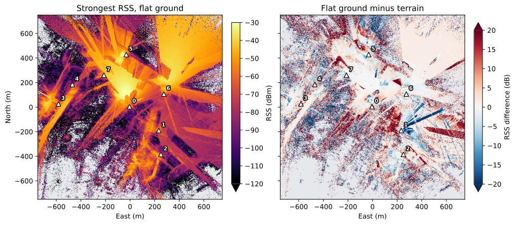
The two versions differ in the ground and in the materials. Flat ground moves the transmitters up or down by up to 8 m here, and the flat version makes the ground and the buildings concrete, where the terrain version has surface classes and metal roofs. On flat ground, 83.4% of the cells are reached, against 79.2% with terrain. Where both reach a cell, the median difference is +1.2 dB. Where the terrain RSS is at least -90 dBm, in 71% of these cells, the median difference in magnitude is 2.3 dB; below -90 dBm it is 11.7 dB.
Notes#
Conventions. The
conventionsblock ofdataset_manifest.jsonstates the row order, units, no-data values and data types of the arrays. Radio and terrain arrays run south to north;2D_Building_Height_Map.npyand the voxel depth run north to south. The building rasters, the height map and the voxel products sample the cell centres. A radio value is the area-weighted mean of the cell’s two triangles, placed at the cell centre (sample_layoutcell_average).Stored precision. The path gain is stored in 0.01 dB steps, at most 0.005 dB off the solver’s value. RSS and SINR are derived from it on loading.
Other readers. Without OpenWorld Radio Twin, the path gain unpacks with NumPy alone and the index opens with any Parquet reader; the dataset guide gives the formulas. The PyTorch dataset reads the same arrays as tensors; the tutorial Radio maps as a PyTorch dataset shows how.