OpenWorld Radio Twin: Interactive, Information-Rich RF Research Generation from Open Data

Only the import changes

A geographic scene loads like a Sionna file scene. The returned object is a native sionna.rt.Scene; arrays, radio devices, solvers, radio maps, rendering and preview stay the upstream API.

# Sionna file scene
from sionna.rt import load_scene
scene = load_scene(filename)

# Geographic scene: same call, WGS84 coordinates
from openworld_radio_twin.rt import load_scene
scene = load_scene(latitude=52.3762, longitude=4.8993, radius_m=250)

From a point on the globe to a Sionna scene

Four environmental layers from open geodata, compiled into one metric frame with the receiver surface and the radio outputs.

1

Compile

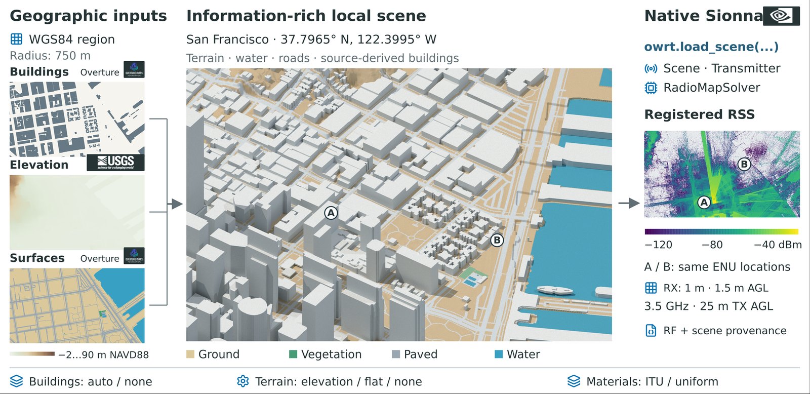
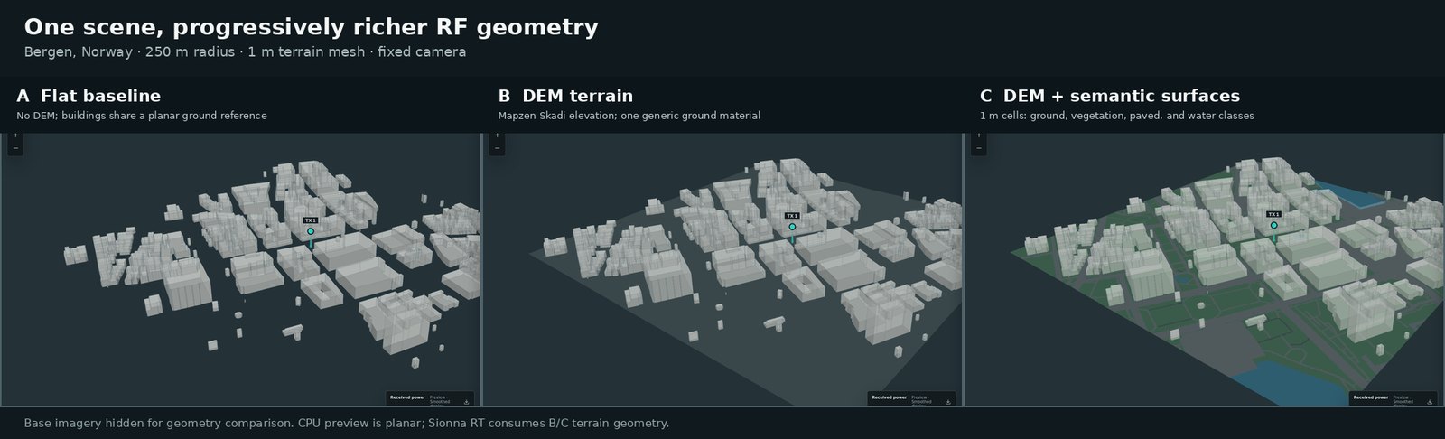
Buildings from Overture and OpenStreetMap worldwide, or from 3DBAG, Berlin LoD2 and Boston BPDA models by region; bare-earth terrain from USGS 3DEP or Mapzen; water levelled per component; ground, vegetation, paved and water classes with ITU material proxies.

2

Simulate

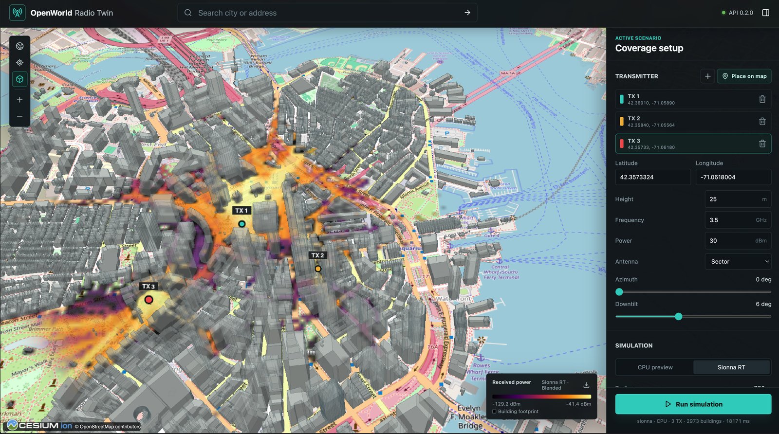
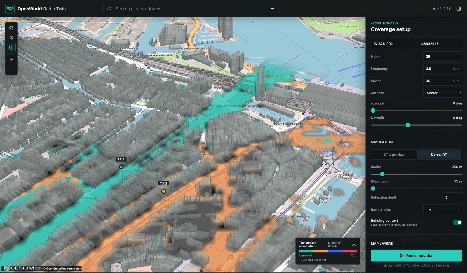
The scene is plain Mitsuba XML and PLY. Sionna RT solves radio maps on a terrain-following measurement surface and channel responses with PathSolver. The explorer places transmitters inside the compiled scene and drapes the result on its terrain; a CPU preview shares the same output contract.

3

Generate

One scene expands into seeded cases with per-case transmitter layouts and solver settings. Datasets resume after interruption, extend deterministically, and record the source, release and resolution behind every array.

What each layer changes

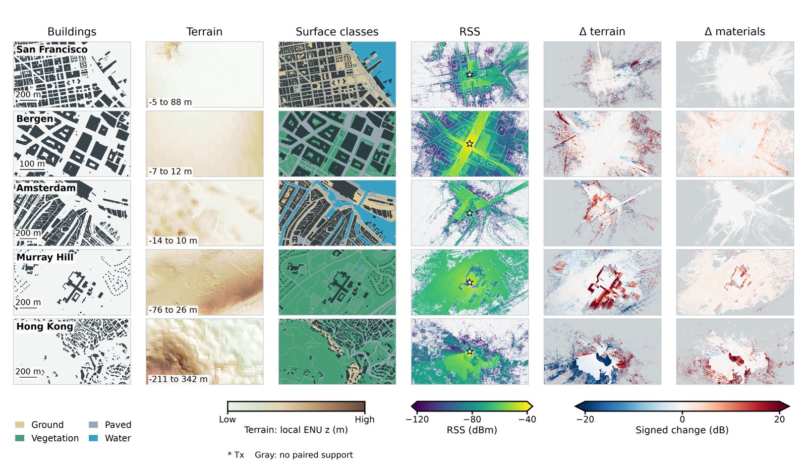
Controlled comparisons on the same scene, transmitter and seed. Only one layer changes at a time.

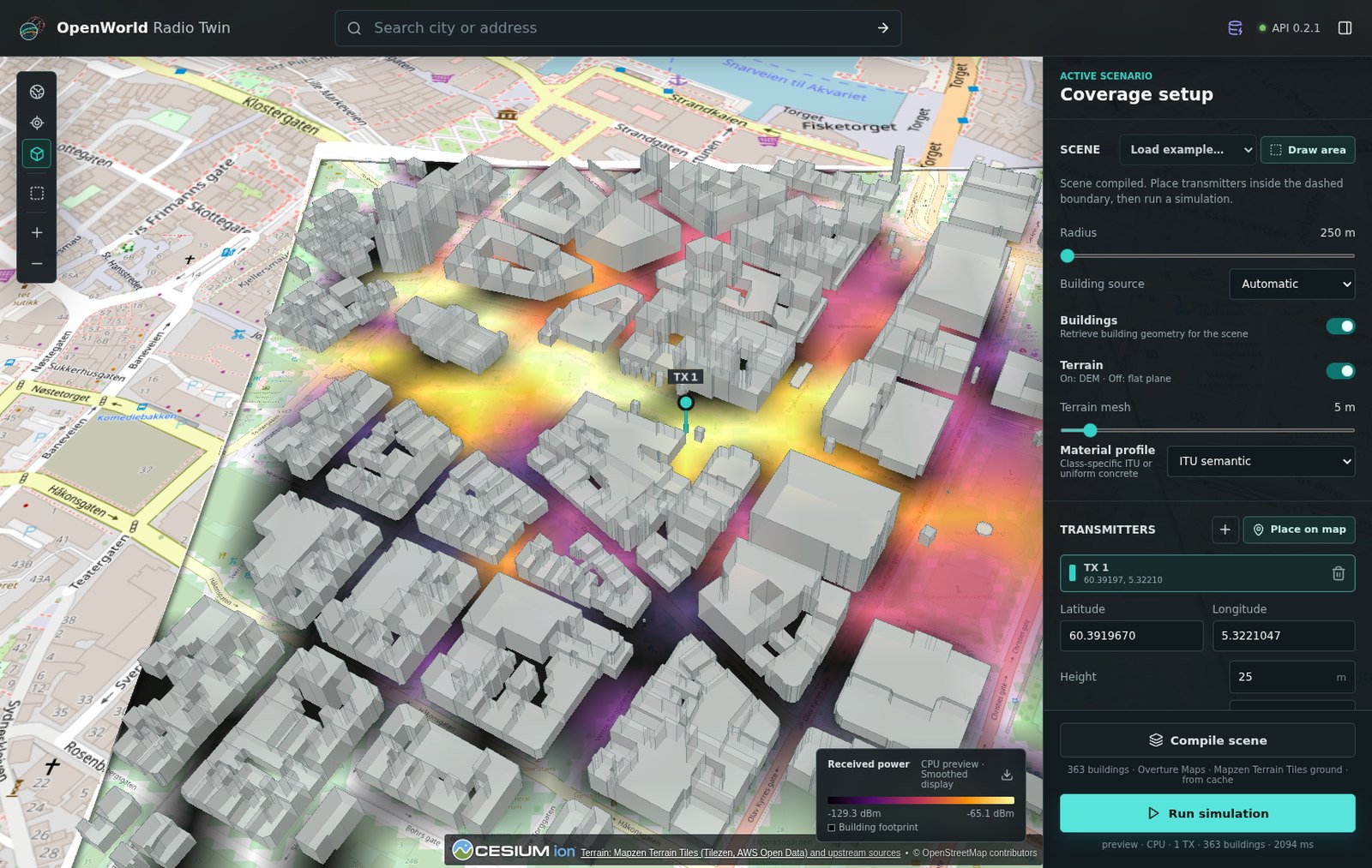
A compiled Bergen scene shown as an inset of the globe in the interactive explorer — **Scene first, then transmitters.** The explorer compiles the drawn square through the same cache as `load_scene` and shows it as an inset of the globe: scene terrain, surface classes and buildings inside the dashed boundary, display terrain outside.

Five-city terrain and material sensitivity comparison — **Terrain and materials at five sites.** Aligned scene layers, received signal strength, and signed changes from the controlled terrain and material experiments. Gray cells lack paired positive RSS.

Bergen scene as flat baseline, terrain mesh, and terrain with semantic surfaces — **The same Bergen scene three ways.** Flat ground, the elevation-following mesh with one material, and the same mesh split into ground, vegetation, paved and water surfaces.

Transmitter association map over Amsterdam with two transmitters — **Multi-cell association in Amsterdam.** Two transmitters and 5,000 dynamically loaded buildings; colour marks the serving transmitter under the configured association criterion.

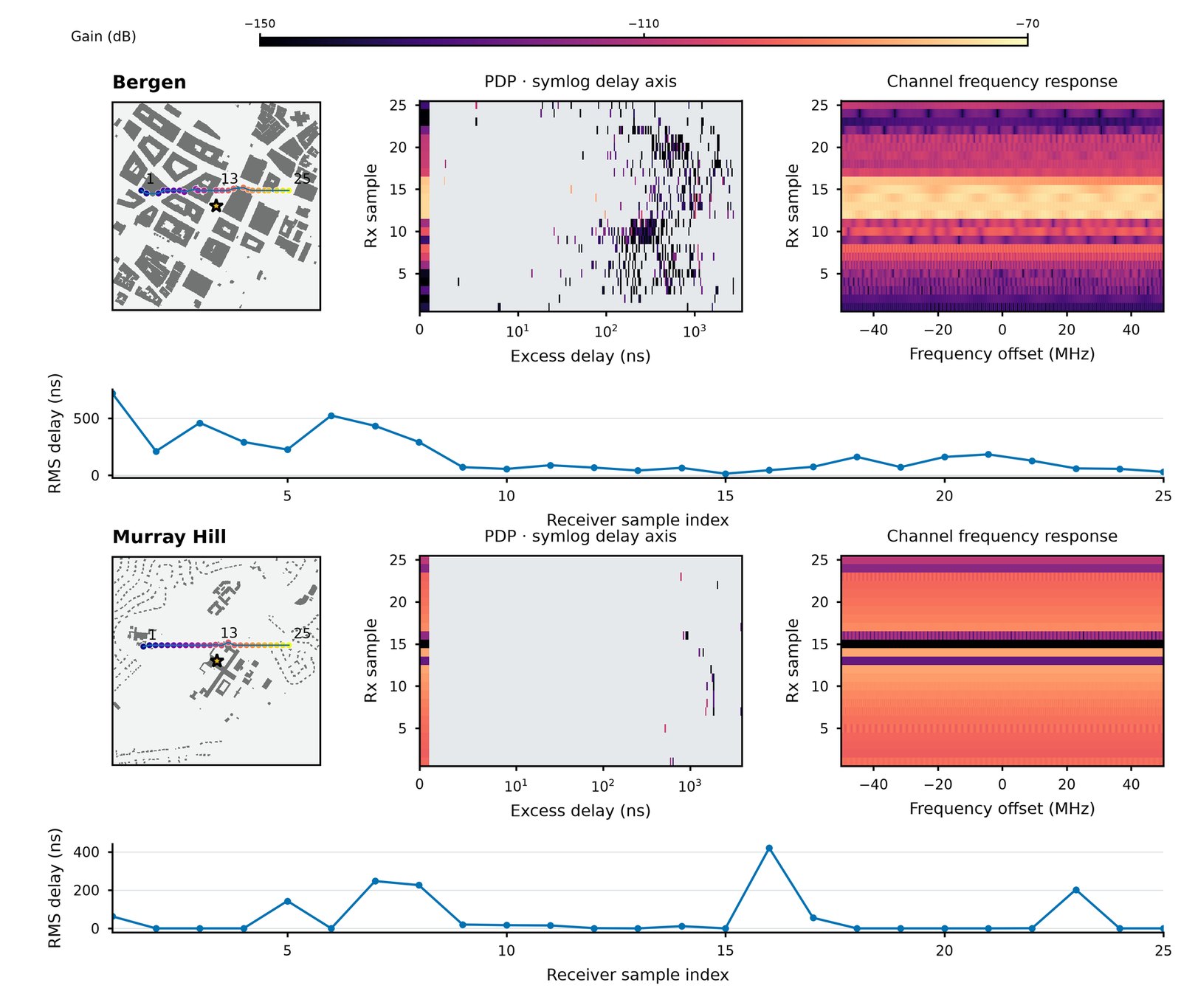
Power-delay profiles, RMS delay spread and channel frequency responses — **Beyond coverage maps.** Native `PathSolver` outputs on OWRT scenes in Bergen and Murray Hill: power-delay profiles, RMS delay spread and channel frequency responses.

Sionna RT RSS maps at 100, 10, 5, 2 and 1 metre cell sizes — **Native resolution.** The same Boston scene from 100 m down to 1 m cells; pixels are copied from native solver cells, never interpolated.

Exported products from one Boston run

Received signal strength export — Received power (dBm)

Transmitter association export — Transmitter association

Receiver-height voxel occupancy slice — Receiver-height voxel slice

Maximum occupied voxel elevation preview — Voxel z-depth preview

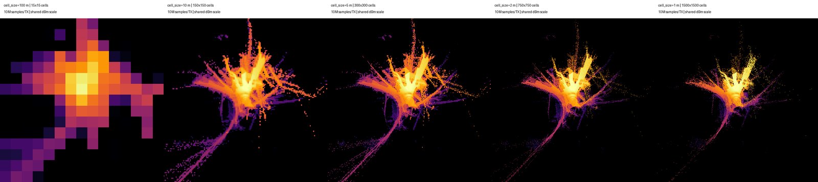
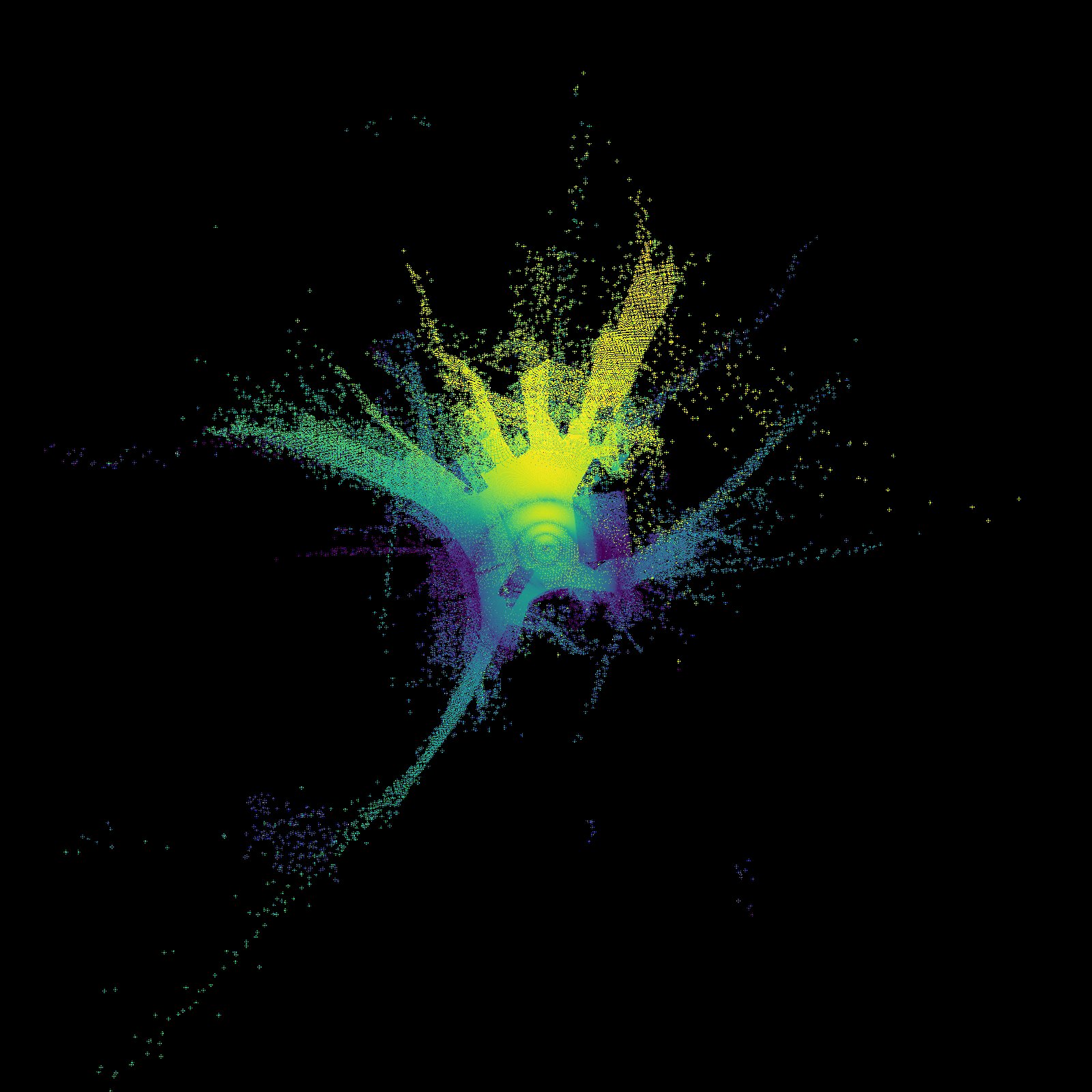
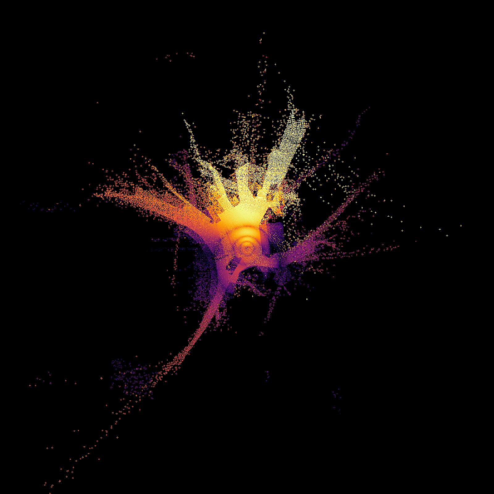
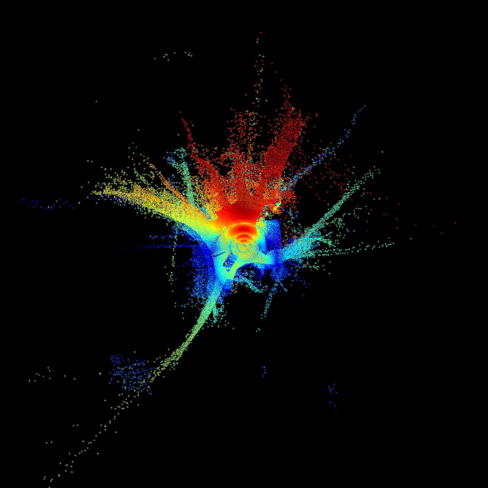
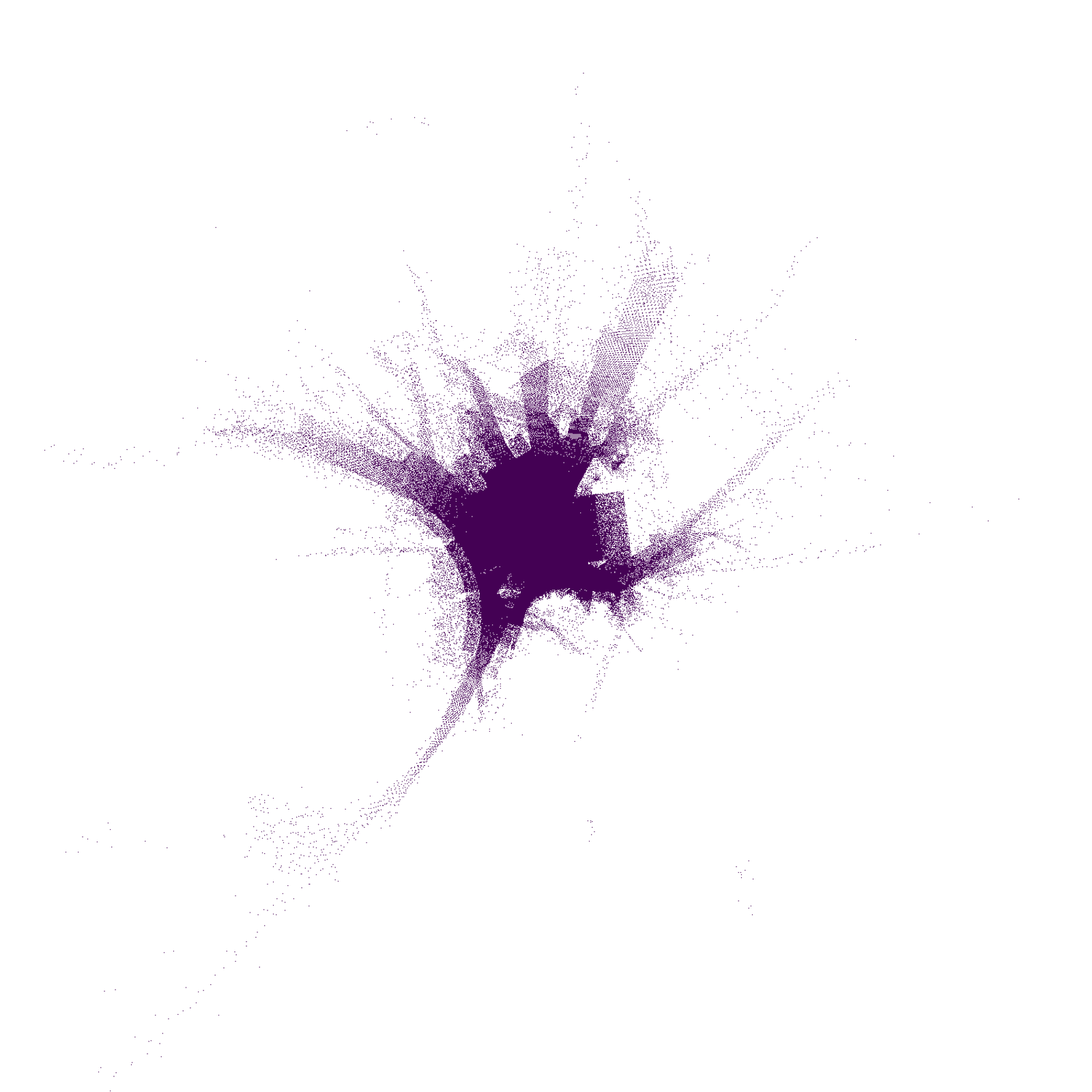
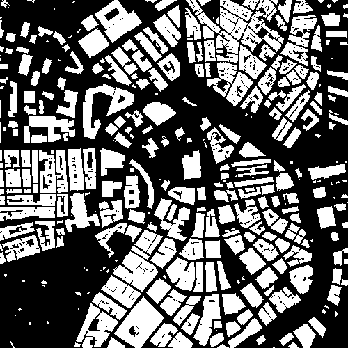
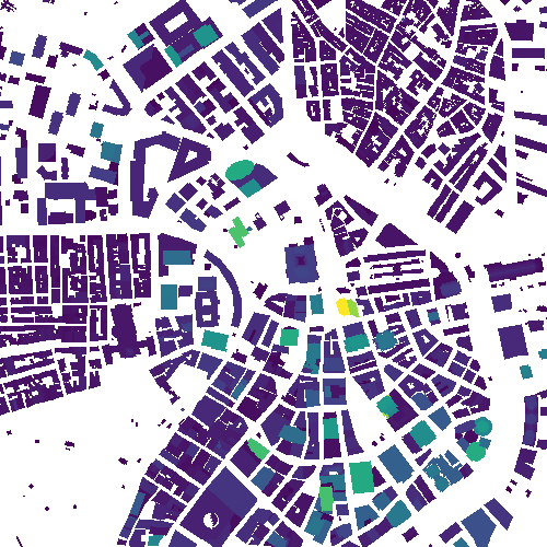
One 1,500 m × 1,500 m scene, one 3.5 GHz sector transmitter, 1 m cells, 1.5 m receiver plane. PNGs keep one pixel per solver cell with transparent no-data; raw arrays ship alongside.

Features

Continuous globe

A CesiumJS world with display terrain everywhere. Drag a diagonal to define a scene; the compiled scene replaces the globe inside its square, with its own terrain, surfaces and buildings, and transmitters are placed inside it.

Buildings at source detail

Overture and OSM extrusions worldwide; native LoD2 roofs from 3DBAG, Berlin and Boston selected automatically by location, or by explicit ID.

Auditable terrain

Bare-earth DEMs from USGS 3DEP and Mapzen Skadi with source, model and local elevation arrays kept apart; water levelled and recorded.

Semantic surfaces

Non-overlapping ground, vegetation, paved and water meshes with documented ITU material proxies, each switchable at solve time.

Sionna-native

Terrain-following measurement surfaces, native propagation controls, path solvers and rendering on the same scene. The CPU preview shares the same output contract.

Reproducible datasets

Seeded expansion with PCG64, per-case provenance, resume after interruption, deterministic extension, and selective artifacts.

Get started

# install
git clone https://github.com/zhiheng-yang/openworld-radio-twin.git
cd openworld-radio-twin
./scripts/setup.sh
conda activate owrt

# interactive explorer
./scripts/run.sh          # http://127.0.0.1:8765

# compile a reusable scene
owrt scene compile --lat 52.3762 --lon 4.8993 --radius 250 --output scenes/amsterdam

from openworld_radio_twin import rt as owrt
from sionna.rt import PlanarArray, RadioMapSolver, Transmitter

scene = owrt.load_scene(latitude=52.3762, longitude=4.8993, radius_m=250)
scene.tx_array = PlanarArray(num_rows=1, num_cols=1, pattern="iso", polarization="V")
scene.rx_array = PlanarArray(num_rows=1, num_cols=1, pattern="iso", polarization="V")
scene.add(Transmitter(name="tx", position=owrt.position(
    scene, latitude=52.3770, longitude=4.9003, height_agl=25.0)))

radio_map = RadioMapSolver()(
    scene, measurement_surface=owrt.measurement_surface(scene, cell_size=(5.0, 5.0)))

Read the quickstart

BibTeX

@software{yang2026openworldradiotwin,
  author  = {Zhiheng Yang},
  title   = {OpenWorld Radio Twin: Interactive World-Scale Wireless Digital Twins},
  year    = {2026},
  version = {0.2.1},
  url     = {https://github.com/zhiheng-yang/openworld-radio-twin},
  license = {Apache-2.0}
}